Fitts D.D. - Principles of Quantum Mechanics[c] As Applied to Chemistry and Chemical Physics (1999)(en)

112	Harmonic oscillator
	N^ ^ayjëii ^ay(N^ 1)jëii ^ay(ë 1)jëii (ë 1)^ayjëii	(4:28)

where equations (4.23) and (4.26b) have been used. In this case we see that

j	ëi	i		^		1. The operator ^ay changes
^ay			is an eigenfunction of N^ with eigenvalue ë
the eigenstate jëii to an eigenstate of				N with a higher value, ë 1, of the

eigenvalue. The energy of the oscillator is increased by "ù. Thus, the operator

^ay is called a raising operator or a creation operator.

Quantization of the energy

In the determination of the energy eigenvalues, we ®rst show that the

eigenvalues ë of ^ are positive (ë > 0). Since the expectation value of the

N

operator ^ for an oscillator in state jë i is ë, we have

N i

hë j ^ jë i ëhë jë i ë i N i i i

^

The integral hëijNjëii may also be transformed in the following manner

h j j

i h

j

j

i

…

…j

^aöëi

j

2 dô

ëi N^ ëi

ëi

^ay^a ëi

(^aöëi)(^aöëi) dô

The integral on the right

must be

positive, so

that

ë is

positive and the

^

^

eigenvalues of N and H cannot be negative.

For the condition ë 0, we have

which requires that

…j^aöëij2 dô 0

^aj(ë 0)ii 0

(4:29)

For eigenvalues ë greater than zero, the quantity ^ajëii is non-vanishing.

To ®nd further restrictions on the values of ë, we select a suitably large, but otherwise arbitrary value of ë, say ç, and continually apply the lowering operator ^a to the eigenstate jçii, thereby forming a succession of eigenvectors

^ajçii, ^a2jçii, ^a3jçii, . . .

with respective eigenvalues ç ÿ 1, ç ÿ 2, ç ÿ 3, . . . We have already shown

that if jçii is an eigenfunction of	^	^ajçii	2is also an eigenfunction. By
	N, then
	^		jçii is an eigenfunction, and
iteration, if ^ajçii is an eigenfunction of N, then ^a

so forth, so that the members of the sequence are all eigenfunctions. Eventually this procedure gives an eigenfunction ^ak jçii with eigenvalue (ç ÿ k), k being a positive integer, such that 0 < (ç ÿ k) , 1. The next step in the sequence would yield the eigenfunction ^ak 1jçii with eigenvalue ë (ç ÿ k ÿ 1) , 0, which is not allowed. Thus, the sequence must terminate by the condition

^ak 1jçii ^a[^ak jçii] 0

4.2 Quantum treatment

113

The only circumstance in which ^a operating on an eigenvector yields the value zero is when the eigenvector corresponds to the eigenvalue ë 0, as shown in equation (4.29). Since the eigenvalue of ^ak jçii is ç ÿ k and this eigenvalue equals zero, we have ç ÿ k 0 and ç must be an integer. The minimum value of ë ç ÿ k is, then, zero.

Beginning with ë 0, we can apply the operator ^ay successively to j0ii to form a series of eigenvectors

^ayj0ii, ^ay2j0ii, ^ay3j0ii, . . .

with respective eigenvalues 0, 1, 2, . . . Thus, the eigenvalues of the operator ^

N are the set of positive integers, so that ë 0, 1, 2, . . . Since the value ç was chosen arbitrarily and was shown to be an integer, this sequence generates all

the eigenfunctions of ^ . There are no eigenfunctions corresponding to non-

N

integral values of ë. Since ë is now known to be an integer n, we replace ë by n in the remainder of this discussion of the harmonic oscillator.

The energy eigenvalues as related to ë in equation (4.25) are now expressed

in terms of n by
En (n 21)"ù, n 0, 1, 2, . . .	(4:30)

so that the energy is quantized in units of "ù. The lowest value of the energy or zero-point energy is "ù=2. Classically, the lowest energy for an oscillator is zero.

Non-degeneracy of the energy levels

To determine the degeneracy of the energy levels or, equivalently, of the

eigenvalues of the number operator ^ , we must ®rst obtain the eigenvectors

N

j0ii for the ground state. These eigenvectors are determined by equation (4.29).
When equation (4.18a) is substituted for ^a, equation (4.29) takes the form
	d	î j0ii			d	î ö0i(î) 0
	dî				dî
or
		dö0i		ÿî dî
			ö0i

This differential equation may be integrated to give

ö0i(î) ceÿî2=2 eiáðÿ1=4eÿî2=2

where the constant of integration c is determined by the requirement that the functions öni(î) be normalized and eiá is a phase factor. We have used the standard integral (A.5) to evaluate c. We observe that all the solutions for the ground-state eigenfunction are proportional to one another. Thus, there exists

114	Harmonic oscillator

only one independent solution and the ground state is non-degenerate. If we arbitrarily set á equal to zero so that ö0(î) is real, then the ground-state eigenvector is

	j0i ðÿ1=4eÿî2=2	^	(4:31)
	We next show that if the eigenvalue n of the number operator		is non-
		N

degenerate, then the eigenvalue n 1 is also non-degenerate. We begin with the assumption that there is only one eigenvector with the property that

^ j i j i

N n n n

and consider the eigenvector j(n 1)ii, which satis®es

^ j( 1) i ( 1)j( 1) i

N n i n n i

If we operate on j(n 1)ii with the lowering operator ^a, we obtain to within a multiplicative constant c the unique eigenfunction jni,

^aj(n 1)ii cjni

We next operate on this expression with the adjoint of ^a to give

^y^j( 1) i ^ j( 1) i ( 1)j( 1) i ^yj i a a n i N n i n n i ca n

from which it follows that

j(n 1)ii n c 1 ^ayjni

Thus, all the eigenvectors j(n 1)ii corresponding to the eigenvalue n 1 are proportional to ^ayjni and are, therefore, not independent since they are proportional to each other. We conclude then that if the eigenvalue n is nondegenerate, then the eigenvalue n 1 is non-degenerate.

Since we have shown that the ground state is non-degenerate, we see that the next higher eigenvalue n 1 is also non-degenerate. But if the eigenvalue n 1 is non-degenerate, then the eigenvalue n 2 is non-degenerate. By iteration, all

of the eigenvalues of ^ are non-degenerate. From equation (4.30) we observe n N

that all the energy levels En of the harmonic oscillator are non-degenerate.

4.3 Eigenfunctions

Lowering and raising operations

From equations (4.27) and (4.28) and the conclusions that the eigenvalues of ^

N

^	j	i	and ^ay	j	n	i	are
are non-degenerate and are positive integers, we see that ^a n
eigenfunctions of N with eigenvalues n ÿ 1 and	n 1, respectively. Accor-
dingly, we may write
^ajni cnjn ÿ 1i				(4:32a)

4.3 Eigenfunctions	115
and
^ayjni c9njn 1i	(4:32b)

where cn and c9n are proportionality constants, dependent on the value of n, and to be determined by the requirement that jn ÿ 1i, jni, and jn 1i are normalized. To evaluate the numerical constants cn and c9n, we square both sides of

equations (4.32a) and (4.32b) and integrate with respect to î to obtain

…ÿ1j

j

j j

…ÿ1

ÿ

ÿ

1

1

^aön

2 dî

cn

2

ö

n

1

ön

1 dî

(4:33a)

and

…ÿ1j

j

j

j

…ÿ1

1

1

^ayön 2 dî

1

c9n

2

ön

ön

1 dî

(4:33b)

The integral on the left-hand side of equation (4.33a) may be evaluated as follows

1

1

…ÿ1j

^aön

j

2 dî

…ÿ1

(^aön )(^aön) dî

h

n

^ay^a n

n N^

j

n

i

n

j

j

i h j

Similarly, the integral on the left-hand side of equation (4.33b) becomes

1

1

…ÿ1j

^ayön

j

2 dî

…ÿ1

(^ayön )(^ayön) dî

h

n

^^aay

n

i h

n

N^

1 n

n

1

j

j

j

j i

Since the eigenfunctions are normalized, we obtain

jcnj2 n,

jc9nj2 n 1

Without loss of generality, we may let cn and c9n be real and positive, so that

equations (4.32a) and (4.32b) become	ÿ	i	:
^ajni p•••j
pn n		1	(4 34a)
•••••••••••
^ayjni n 1jn 1i			(4:34b)

If the normalized eigenvector jni is known, these relations may be used to obtain the eigenvectors jn ÿ 1i and jn 1i, both of which will be normalized.

Excited-state eigenfunctions

We are now ready to obtain the set of simultaneous eigenfunctions for the

commuting operators ^ and ^ . The ground-state eigenfunction j0i has already

N H

been determined and is given by equation (4.31). The series of eigenfunctions

j1i, j2i, . . . are obtained from equations (4.34b) and (4.18b), which give

jn 1i [2(n 1)]ÿ1=2 î ÿ ddî jni (4:35)

Thus, the eigenvector j1i is obtained from j0i

116				Harmonic oscillator
			d					îeÿî2=2
1	2ÿ1=2 î			(ðÿ1=4eÿî2=2)		21=2	ðÿ1=4
j i		ÿ	dî

the eigenvector j2i from j1i

2

1

î

d

(21=2ðÿ1=4îeÿî2=2)

2ÿ1=2

ðÿ1=4(2î2

1)eÿî2

=2

ÿ dî

ÿ

j i

2

the eigenvector j3i from j2i

			d			1)eÿî2
3	6ÿ1=2 î			(2ÿ1=2ðÿ1=4(2î2			=2)
j i		ÿ dî			ÿ

3ÿ1=2ðÿ1=4(2î3 ÿ 3î)eÿî2=2

and so forth, inde®nitely. Each of the eigenfunctions obtained by this procedure is normalized.

When equation (4.18a) is combined with (4.34a), we have

jn ÿ 1i (2n)ÿ1=2	d	jni
	î dî		(4:36)

Just as equation (4.35) allows one to go `up the ladder' to obtain jn 1i from jni, equation (4.36) allows one to go `down the ladder' to obtain jn ÿ 1i from jni. This lowering procedure maintains the normalization of each of the eigenvectors.

Another, but completely equivalent, way of determining the series of eigenfunctions may be obtained by ®rst noting that equation (4.34b) may be written for the series n 0, 1, 2, . . . as follows

j1i ^ayj0i

j2i 2ÿ1=2^ayj1i 2ÿ1=2(^ay)2j0i j3i 3ÿ1=2^ayj2i (3!)ÿ1=2(^ay)3j0i

...

Obviously, the expression for jni is

jni (n!)ÿ1=2(^ay)nj0i

Substitution of equation (4.18b) for ^ay and (4.31) for the ground-state eigenvector j0i gives

jni (2n n!)ÿ1=2ðÿ1=4	î ÿ	d	neÿî2=2	(4:37)
		dî

This equation may be somewhat simpli®ed if we note that

(4:41)

î ÿ dî eÿî					4.3 Eigenfunctions					ÿ îeî			ÿ eî	117
			=2		î ÿ ddî eî	=2eÿî	2	îeÿî	=2		=2eÿî	2		=2 ddî eÿî			2
	d	2			2			2		2			2

2

d

2

ÿeî

=2

eÿî

dî

so that

d

n

dn

2

2

2

î ÿ

eÿî

=2

(ÿ1)neî

=2

eÿî

dî

dîn

Substitution of equation (4.38) into (4.37) gives

jni (ÿ1)n(2n n!)ÿ1=2ðÿ1=4eî2=2 dn eÿî2 dîn

which may be used to obtain the entire set of eigenfunctions of ^ and ^ .

N H

(4:38)

(4:39)

Eigenfunctions in terms of Hermite polynomials

It is customary to express the eigenfunctions for the stationary states of the harmonic oscillator in terms of the Hermite polynomials. The in®nite set of Hermite polynomials Hn(î) is de®ned in Appendix D, which also derives many of the properties of those polynomials. In particular, equation (D.3) relates the Hermite polynomial of order n to the nth-order derivative which appears in equation (4.39)

Hn(î) (ÿ1)neî2 ddînn eÿî2

Therefore, we may express the eigenvector jni in terms of the Hermite polynomial Hn(î) by the relation

jni ön(î) (2n n!)ÿ1=2ðÿ1=4 Hn(î)eÿî2=2

(4:40)

The eigenstates øn(x) are related to the functions ön(î) by equation (4.16), so that we have

øn(x) (2n n!)ÿ1=2	mù		1=4	2
				Hn(î)eÿî	=2
	ð"

ù 1=2

î m x

"

For reference, the Hermite polynomials for n 0 to n 10 are listed in Table 4.1. When needed, higher-order Hermite polynomials are most easily obtained from the recurrence relation (D.5). If only a single Hermite polynomial is wanted and the neighboring polynomials are not available, then equation (D.4) may be used.

118 Harmonic oscillator

							Table 4.1. Hermite polynomials
n																Hn(î)
0	1
1	2î
	2	ÿ 2
2	4î3
3	8î	4ÿ 12î 2					3 12
4	16î	5	ÿ 48î
5	32î	6	ÿ 160î				4 120î					2	ÿ	3
6	64î		ÿ		480î				720î
7	128î		7	ÿ 1344î				5	3360î						4ÿ 1680î
			8					6									2	1680
8	256î		9	ÿ 3584î				7	13440î						5 ÿ 13440î		3
9	512î			ÿ		9216î				48384î					ÿ	6				4
																80640î			30240î
10	1024î			10		ÿ 23040î				8	161280î ÿ 403200î										302400î	2	ÿ 30240

The functions ön(î) in equation (4.40) are identical to those de®ned by equation (D.15) and, therefore, form a complete set as shown in equation (D.19). Substituting equation (4.16) into (D.19) and applying the relation (C.5b), we see that the functions øn(x) in equation (4.41) form a complete set, so that

X1

øn(x)øn(x9) ä(x ÿ x9)		(4:42)
n 0
Physical interpretation
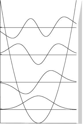
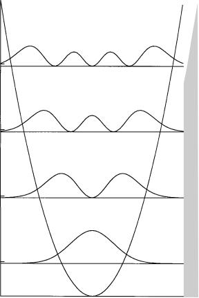
The ®rst four eigenfunctions øn(x) for n 2	0, 1, 2, 3 are plotted in Figure 4.2
and the corresponding functions [øn(x)]	in Figure	4.3. These ®gures also

show the outline of the potential energy V(x) from equation (4.5) and the four corresponding energy levels from equation (4.30). The function [øn(x)]2 is the probability density as a function of x for the particle in the nth quantum state. The quantity [øn(x)]2 dx at any point x gives the probability for ®nding the particle between x and x dx.

We wish to compare the quantum probability distributions with those obtained from the classical treatment of the harmonic oscillator at the same energies. The classical probability density P( y) as a function of the reduced distance y (ÿ1 < y < 1) is given by equation (4.10) and is shown in Figure 4.1. When equations (4.8), (4.14), and (4.30) are combined, we see that the

maximum displacement in terms of î for a classical oscillator with energy
1	p	p		p
(n 2)"ù is	••••••••••••••	••••••••••••••		••••••••••••••
	2n 1.	For î , ÿ 2n 1	and î .	2n 1, the classical

4.3 Eigenfunctions

119

Energy

7 hù

2

5 hù

2

3 hù

2

1 hù

2

V

ø3

n 5 3

ø2

n 5 2

ø1

n 5 1

ø0

n 5 0

x

0

Figure 4.2 Wave functions and energy levels for a particle in a harmonic potential well. The outline of the potential energy is indicated by shading.

probability for ®nding the particle is equal to zero. These regions are shaded in Figures 4.2 and 4.3.

Each of the quantum probability distributions differs from the corresponding classical distribution in one very signi®cant respect. In the quantum solution there is a non-vanishing probability of ®nding the particle outside the classically allowed region, i.e., in a region where the total energy is less than the potential energy. Since the Hermite polynomial Hn(î) is of degree n, the wave function øn(x) has n nodes, a node being a point where a function touches or crosses the x-axis. The quantum probability density [øn(x)]2 is zero at a node. Within the classically allowed region, the wave function and the probability density oscillate with n nodes; outside that region the wave function and probability density rapidly approach zero with no nodes.

120	Harmonic oscillator

Energy

7 hù

2

5 hù

2

3 hù

2

1 hù

2

|ø3|2

n 5 3

|ø2|2

n 5 2

|ø1|2

n 5 1

|ø0|2

n 5 0

x

0

Figure 4.3 Probability densities and energy levels for a particle in a harmonic potential well. The outline of the potential energy is indicated by shading.

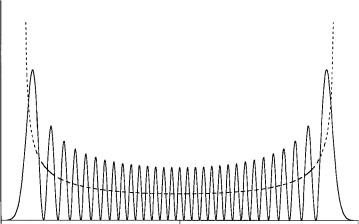
While the classical particle is most likely to be found near its maximum displacement, the probability density for the quantum particle in the ground state is largest at the origin. However, as the value of n increases, the quantum probability distribution begins to look more and more like the classical probability distribution. In Figure 4.4 the function [ø30(x)]2 is plotted along with the classical result for an energy 30:5 "ù. The average behavior of the rapidly oscillating quantum curve agrees well with the classical curve. This observation is an example of the Bohr correspondence principle, mentioned in Section 2.3. According to the correspondence principle, classical mechanics and quantum theory must give the same results in the limit of large quantum numbers.

4.4 Matrix elements

121

|ø30(x)|2

x

0

Figure 4.4 The probability density jø30(x)j2 for an oscillating particle in state n 30. The dotted curve is the classical probability density for a particle with the same energy.

4.4 Matrix elements

In the application to an oscillator of some quantum-mechanical procedures, the matrix elements of xn and ^pn for a harmonic oscillator are needed. In this section we derive the matrix elements hn9jxjni, hn9jx2jni, hn9j^pjni, and hn9j^p2jni, and show how other matrix elements may be determined.

The ladder operators ^a and ^ay de®ned in equation (4.18) may be solved for x and for ^p to give

"

1=2

x

(^ay ^a)

(4:43a)

2mù

"

1=2

^p i

m ù

(^ay ÿ ^a)

(4:43b)

2

From equations

(4.34)

and the

orthonormality of

the

harmonic

oscillator

eigenfunctions

j

i

n , we ®nd that the matrix elements of ^a and ^ay are

n9

^ahy nj

j

ipn

•••1 n9 n

ÿ

1

p•••n

1än9,n 1

(4:44b)

h

j

n9

^a n

pnhn9jn

1i pnän9,nÿ1

(4:44a)

•••••••••••

•••••••••••

j i h j i

The set of equations (4.43) and (4.44) may be used to evaluate the matrix elements of any integral power of x and ^p.

To ®nd the matrix element hn9jxjni, we apply equations (4.43a) and (4.44) to obtain