Fitts D.D. - Principles of Quantum Mechanics[c] As Applied to Chemistry and Chemical Physics (1999)(en)

202 Spin

According to the Biot and Savart law of electromagnetic theory,1 the magnetic ®eld B at the `®xed' electron due to the revolving positively charged

nucleus is given in SI units to ®rst order in v=c by
1	(E 3 vn)
B c2		(7:26)

where E is the electric ®eld due to the revolving nucleus, vn is the velocity of the nucleus relative to the electron, and c is the speed of light. The electric force F is related to E and the potential energy V(r) of interaction between the nucleus and the electron by

F ÿeE ÿ=V
Thus, the electric ®eld at the electron is
E	rn dV(r)				(7:27)
	er		dr

where rn is the vector distance of the nucleus from the electron. The vector r from nucleus to electron is ÿrn and the velocity v of the electron relative to the nucleus is ÿvn. Accordingly, the angular momentum L of the electron is

L r 3 p me(r 3 v) me(rn 3 vn)					(7:28)
Combining equations (7.26), (7.27), and (7.28), we have
1			dV (r)		(7:29)
B				L
	eme c2 r		dr

The spin±orbit energy ÿMs : B may be related to the spin and orbital

angular momenta through equations (7.1) and (7.29)
ÿMs : B	1 dV(r)				L	: S
	m2 c2 r		dr
	e

This expression is not quite correct, however, because of a relativistic effect in changing from the perspective of the electron to the perspective of the nucleus.

The correction,2 known as the Thomas precession, introduces the factor 1										on
									2
the right-hand side to give
ÿMs : B		1				dV(r)		L : S
		2m2 c2 r dr
		e
								^
The corresponding spin±orbit Hamiltonian operator Hso is, then,
^		1		dV(r)			^	: ^
Hso 2me2 c2 r				dr			L	S	(7:30)

1R. P. Feyman, R. B. Leighton, and M. Sands (1964) The Feynman Lectures on Physics, Vol. II (AddisonWesley, Reading, MA) section 14-7.

2 J. D. Jackson (1975) Classical Electrodynamics, 2nd edition (John Wiley & Sons, New York) pp. 541±2.

7.4 Spin±orbit interaction

203

For a hydrogen atom, the potential energy V (r) is given by equation (6.13)

with Z 1 and	^
	Hso becomes		^		^	: ^			(7:31)
where			Hso		î(r)L	S
		î(r)			e2				(7:32)
				8ðå0 me2 c2 r3
					^
Thus, the total Hamiltonian operator H for a hydrogen atom including spin±
orbit coupling is
	^	^	^		^	^		: ^	(7:33)
	H H0		Hso		H0	î(r)L		S

where	^	is the Hamiltonian operator for the hydrogen atom without the
	H0

inclusion of spin, as given in equation (6.14).

The effect of the spin±orbit interaction term on the total energy is easily shown to be small. The angular momenta jLj and jSj are each on the order of " and the distance r is of the order of the radius a0 of the ®rst Bohr orbit. If we also neglect the small difference between the electronic mass me and the reduced mass ì, the spin±orbit energy is of the order of

8ðåe2"22 2 3 á2jE1j 0 me c a0

where jE1j is the ground-state energy for the hydrogen atom with Hamiltonian

operator	^	as given by equation (6.57) and á is the ®ne structure constant,
	H0
de®ned by
		á	e2	"				1
			4ðå0	"c		me ca0		137:036

Thus, the spin±orbit interaction energy is about 5 3 10ÿ5 times smaller than

jE1j.

^

for the hydrogen atom in the absence of

While the Hamiltonian operator H0

^

^

the spin±orbit coupling term commutes with L and with

S, the total Hamilto-

nian

operator

^

in

equation (7.33)

does not commute with either

^

^

H

L or

S

^

: ^

because of the presence of the scalar product L

S. To illustrate this feature,

^

^

:

^

^

^

: ^

we consider the commutators [Lz

, L

S] and [Sz, L

S],

^

^

: ^

^

^

^

^ ^

^

^

^ ^

^

^ ^

^

[Lz,

L

S]

[Lz, (Lx Sx Ly S y

Lz Sz)] [Lz, Lx]Sx

[Lz, Ly]S y 0

^

^

^

^

(7:34)

i"(Ly Sx ÿ Lx S y) 60

^

^

: ^

^ ^

^

^ ^

^

^

^

^ ^

60

(7:35)

[Sz,

L

S]

[Sz,

Sx]Lx [Sz, S y]Ly

i"(Lx S y

ÿ Ly Sx)

where equations (5.10) and (7.2) have been used. Similar expressions apply to

the other components of	^	^
	L and	S. Thus, the vectors L and S are no longer

204	Spin
	^2	^2	^	: ^
constants of motion. However, the operators L		and S	do commute with L	S,

which follows from equations (5.15), so that the quantities L2 and S2 are still constants of motion.

We now introduce the total angular momentum J, which is the sum of L

and S
					J L S				(7:36)
^	and	^2	commute with			^	. The addition of equations (7.34)
The operators J		J				H0
and (7.35) gives
	^	^	: ^	^	^ :	^	^	^	: ^
	[Jz, L		S] [Lz, L			S] [Sz, L			S] 0

The addition of similar relations for the x- and y-components of these angular

^

^

: ^

^

^

: ^

momentum vectors leads to the result that [J,

L

S] 2

0, so that J and L

S

^

commutes with

^

: ^

commute. Furthermore, we may easily show that J

L

S

because each term in

^2

^2

^2

2

^

: ^

commutes with

^

: ^

^

J

L

S

^2

commute with

^

L

S

2

L

S. Thus, J

and J

H

in equation (7.33) and J and J

are constants of

motion.

That the quantities L2, S2, J2, and J are constants of motion, but L and S are not, is illustrated in Figure 7.1. The spin magnetic moment Ms, which is antiparallel to S, exerts a torque on the orbital magnetic moment M, which is antiparallel to L, and alters its direction, but not its magnitude. Thus, the orbital angular momentum vector L precesses about J and L is not a constant of motion. However, since the magnitude of L does not change, the quantity L2 is a constant of motion. Likewise, the orbital magnetic moment M exerts a torque on Ms, causing S to precess about J. The vector S is, then, not a constant of

S

J

L

Figure 7.1 Precession of the orbital angular momentum vector L and the spin angular momentum vector S about their vector sum J.

7.4 Spin±orbit interaction

205

motion, but S2 is. Since J is ®xed in direction and magnitude, both J and J2

are constants of motion.

If we form the cross product

^

^

J 3 J and substitute equations (7.36), (5.11),

and (7.3), we obtain

^ ^

^

^

^

^

^ ^

^ ^

^

^

^

J 3 J (L S) 3 (L S)

(L 3 L) (S 3 S)

i"L

i"S

i"J

where

the

cross

terms

^

^

^

^

each

other. Thus, the

(L

3 S)

and (S 3 L) cancel

^

obeys equation (5.12) and the quantum-mechanical treatment of

operator J

Section 5.2 applies to the total angular momentum. Since

^

^

^

Jx, J y, and Jz each

^2

^

commute with J

but do not commute with one another, we select Jz and seek

the

simultaneous eigenfunctions

j

nlsjm

ji

of the set of mutually commuting

^

2

S

2

,

J

2

, and

^

operators H, L ,

Jz

^

(7:37a)

Hjnlsjmji Enjnlsjmji

^2

jnlsjmji l(l

2

jnlsjmji

(7:37b)

L

1)"

^2

jnlsjmji s(s

2

(7:37c)

S

1)" jnlsjmji

^2

jnlsjmji j(j

2

(7:37d)

J

1)" jnlsjmji

^

mj ÿj, ÿj 1, . . . ,

j

ÿ 1, j

(7:37e)

Jzjnlsjmji mj"jnlsjmji,

From the expression

^

^

^

Jzjnlsjmji (Lz Sz)jnlsjmji (m ms)"jnlsjmji

obtained from (7.36), (5.28b), and (7.5), we see that

mj m ms

(7:38)

The quantum number j takes on the values

l s, l s ÿ 1, l s ÿ 2, . . . , jl ÿ sj

The argument leading to this conclusion is somewhat complicated and may be found elsewhere.3 In the application being considered here, the spin s equals 12

and the quantum number j can have only two values

j l 21

(7:39)

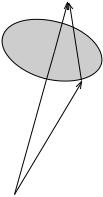
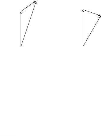
The resulting vectors J are shown in Figure 7.2.

The scalar product

^

: ^

L

S in equation (7.33) may be expressed in terms of

^

operators that commute with H by

^

: ^

1 ^

^

:

^

^

1^

: ^

1^ :

^

1 ^2

^2

^2

) (7:40)

L

S

2(L S)

(L S) ÿ

2L

L ÿ

2S

S

2(J

ÿ L

ÿ S

3B. H. Brandsen and C. J. Joachain (1989) Introduction to Quantum Mechanics (Addison Wesley Longman, Harlow, Essex), pp. 299, 301; R. N. Zare (1988) Angular Momentum (John Wiley & Sons, New York), pp. 45±8.

206		Spin
		S
		S
		J
	L	L
		J

j 5 l 1	1	j 5 l 2	1
	2		2

Figure 7.2 The total angular momentum vectors J obtained from the sum of L and S for s 12 and s ÿ12.

^

so that H becomes

^

^

1

^2

^2

^2

)

(7:41)

H

H0

2î(r)(J

ÿ L

ÿ S

Equation (7.37a) then takes the form

^

1

2

î(r)[ j(j

1)

ÿ l(l 1) ÿ s(s 1)]gjnlsjmji Enjnlsjmji

(7:42)

or

fH0

2"

l"2

H^ 0

î(r) jn, l, 21, l 21, mji Enjn, l, 21, l 21, mji if j l 21

2

(7:43a)

H^

ÿ

(l 1)"2

î(r)

j

n, l,

1, l

ÿ

1, m

ji

E

nj

n, l,

1, l

ÿ

1, m

ji

0

2

ÿ2

2

ÿ2

2

if j l ÿ 12 (7:43b) where equations (7.37b), (7.37c), (7.37d), and (7.39) have also been introduced.

Since the spin±orbit interaction energy is small, the solution of equations (7.43) to obtain En is most easily accomplished by means of perturbation theory, a technique which is presented in Chapter 9. The evaluation of En is left as a problem at the end of Chapter 9.

Problems

7.1Determine the angle between the spin vector S and the z-axis for an electron in spin state jái.

7.2Prove equation (7.19) from equations (7.15) and (7.17).

Problems

207

7.3Show that the pair of operators ó y, ó z anticommute.

7.4Using the Pauli spin matrices in equation (7.25) and the spinors in (7.13),

(a) construct the operators ó and ó corresponding to ^ and ^

ÿ S Sÿ

(b) operate on jái and on jâi with ó 2, óz, ó , óÿ, óx, and ó y and compare the results with equations (7.14), (7.15), (7.16), and (7.17).

7.5Using the Pauli spin matrices in equation (7.25), verify the relationships in (7.19) and (7.22).

8

Systems of identical particles

The postulates 1 to 6 of quantum mechanics as stated in Sections 3.7 and 7.2 apply to multi-particle systems provided that each of the particles is distinguishable from the others. For example, the nucleus and the electron in a hydrogen-like atom are readily distinguishable by their differing masses and charges. When a system contains two or more identical particles, however, postulates 1 to 6 are not suf®cient to predict the properties of the system. These postulates must be augmented by an additional postulate. This chapter introduces this new postulate and discusses its consequences.

8.1 Permutations of identical particles

Particles are identical if they cannot be distinguished one from another by any intrinsic property, such as mass, charge, or spin. There does not exist, in fact and in principle, any experimental procedure which can identify any one of the particles. In classical mechanics, even though all particles in the system may have the same intrinsic properties, each may be identi®ed, at least in principle, by its precise trajectory as governed by Newton's laws of motion. This identi®cation is not possible in quantum theory because each particle does not possess a trajectory; instead, the wave function gives the probability density for ®nding the particle at each point in space. When a particle is found to be in some small region, there is no way of determining either theoretically or experimentally which particle it is. Thus, all electrons are identical and therefore indistinguishable, as are all protons, all neutrons, all hydrogen atoms with 1H nuclei, all hydrogen atoms with 2H nuclei, all helium atoms with 4He nuclei, all helium atoms with 3He nuclei, etc.

Two-particle systems

For simplicity, we ®rst consider a system composed of two identical particles

208

8.1 Permutations of identical particles

209

of mass m. If we label one of the particles as particle 1 and the other as particle

	^
2, then the Hamiltonian operator H(1, 2) for the system is
^		p^2		p^2
		1		2
H(1, 2)	2m		2m V(q1, q2)			(8:1)
where qi (i 1, 2) represents		the	three-dimensional (continuous)			spatial

coordinates ri and the (discrete) spin coordinate ói of particle i. In order for these two identical particles to be indistinguishable from each other, the Hamiltonian operator must be symmetric with respect to particle interchange, i.e., if the coordinates (both spatial and spin) of the particles are interchanged,

^ (1, 2) must remain invariant

H

		^		^
		H(1, 2)		H(2, 1)
If	^	^		then the corresponding SchroÈdinger
	H(1, 2) and	H(2, 1) were to differ,

equations and their solutions would also differ and this difference could be used to distinguish between the two particles.

The time-independent SchroÈdinger equation for the two-particle system is

^	EíØí(1, 2)	(8:2)
H(1, 2)Øí(1, 2)

where í delineates the various states. The notation Øí(1, 2) indicates that the ®rst particle has coordinates q1 and the second particle has coordinates q2. If we exchange the two particles so that particles 1 and 2 now have coordinates q2 and q1, respectively, then the SchroÈdinger equation (8.2) becomes

^		^	(1, 2)Øí(2, 1)	EíØí(2, 1)	(8:3)
H(2, 1)Øí(2, 1)		H
where we have noted that	^
	H(1, 2) is symmetric. Equation (8.3) shows that

Ø (2, 1) is also an eigenfunction of ^ (1, 2) belonging to the same eigenvalue

í H

Eí. Thus, any linear combination of Øí(1, 2) and Øí(2, 1) is also an eigen-

function of ^ (1, 2) with eigenvalue . For simplicity of notation in the

H Eí

following presentation, we omit the index í when it is clear that we are referring to a single quantum state.

The eigenfunction Ø(1, 2) has the form of a wave in six-dimensional space. The quantity Ø (1, 2)Ø(1, 2) dr1 dr2 is the probability that particle 1 with spin function ÷1 is in the volume element dr1 centered at r1 and simultaneously particle 2 with spin function ÷2 is in the volume element dr2 at r2. The product Ø (1, 2)Ø(1, 2) is, then, the probability density. The eigenfunction Ø(2, 1) also has the form of a six-dimensional wave. The quantity Ø (2, 1)Ø(2, 1) is the probability density for particle 2 being at r1 with spin function ÷1 and simultaneously particle 1 being at r2 with spin function ÷2. In general, the two eigenfunctions Ø(1, 2) and Ø(2, 1) are not identical. As an example, if Ø(1, 2) is

210	Systems of identical particles
Ø(1,		2) eÿar1 eÿbr2 (br2 ÿ 1)
where r1 jr1j and r2 jr2j, then Ø(2, 1) would be
Ø(2, 1)		eÿar2 eÿbr1 (br	1) Ø(1, 2)
		1 ÿ	6

Thus, the probability density of the pair of particles depends on how we label the two particles. Since the two particles are indistinguishable, we conclude that neither Ø(1, 2) nor Ø(2, 1) are desirable wave functions. We seek a wave function that does not make a distinction between the two particles and, therefore, does not designate which particle is at r1 and which is at r2.

	To that end, we now introduce the linear hermitian							^
							exchange operator P,
	which has the property
			^	(1, 2) f (2, 1)				(8:4)
			P f				^
	where f (1, 2)	is an	arbitrary	function		of q1 and		operates on
							q2. If P
	^
	H(1, 2)Ø(1, 2), we have
	^ ^		^			^	^	^
	P[H(1, 2)Ø(1, 2)]		H(2, 1)Ø(2, 1)			H(1, 2)Ø(2, 1) H(1, 2)PØ(1, 2)
								(8:5)
	where we have used the fact that			^
				H(1, 2) is symmetric. From equation (8.5) we
	^	^
	see that P and	H(1, 2) commute
			^		^			(8:6)
			[P,		H(1, 2)] 0,
			^		^
	Consequently, the operators P and				H(1, 2) have simultaneous eigenfunctions.

				^
If Ö(1, 2) is an eigenfunction of P, the corresponding eigenvalue ë is given
by
				^					(8:7)
We then have			PÖ(1, 2) ëÖ(1, 2)
^2	Ö(1, 2)	^ ^		^		^		2	(8:8)
P		P[PÖ(1, 2)]		P[ëÖ(1, 2)] ëPÖ(1, 2) ë Ö(1, 2)
Moreover, operating on Ö(1, 2) twice in succession by							^	returns the	two
							P
particles to their original order, so that
		^2		^	Ö(1, 2)				(8:9)
		P	Ö(1, 2) PÖ(2, 1)
				^	2		2		^
From equations (8.8) and (8.9), we see that P						1 and that ë		1. Since P is
hermitian, the eigenvalue ë is real and we obtain ë 1.
There are		only two functions which are simultaneous					eigenfunctions of
^		^
H(1, 2) and		P with respective eigenvalues E and 1. These functions are the
combinations
		ØS 2ÿ1=2[Ø(1, 2) Ø(2, 1)]						(8:10a)
		ØA 2ÿ1=2[Ø(1, 2) ÿ Ø(2, 1)]						(8:10b)
which satisfy the relations

8.1 Permutations of identical particles	211
^	(8:11a)
PØS ØS
^	(8:11b)
PØA ÿØA

The factor 2ÿ1=2 in equations (8.10) normalizes ØS and ØA if Ø(1, 2) is normalized. The combination ØS is symmetric with respect to particle interchange because it remains unchanged when the two particles are exchanged. The function ØA, on the other hand, is antisymmetric with respect to particle interchange because it changes sign, but is otherwise unchanged, when the particles are exchanged.

The functions ØA and ØS are orthogonal. To demonstrate this property, we note that the integral over all space of a function of two or more variables must

be independent of the labeling of those variables
…	… f (x1, . . . , xN ) dx1 . . . dxN … … f (y1, . . . , yN ) dy1 . . . d yN	(8:12)
In particular, we have
or	…… f (1, 2) dq1 dq2 …… f (2, 1) dq1 dq2
	hØ(1, 2)jØ(2, 1)i hØ(2, 1)jØ(1, 2)i
		(8:13)

where f (1, 2) Ø (1, 2)Ø(2, 1). Application of equation (8.13) to hØS jØAi gives

^ ^	(8:14)
hØS jØAi hPØS jPØAi

Applying equations (8.11) to the right-hand side of (8.14), we obtain hØS jØAi ÿhØS jØAi

Thus, the scalar product hØS jØAi must vanish, showing that ØA and ØS are orthogonal.

If the wave function for the system is initially symmetric (antisymmetric), then it remains symmetric (antisymmetric) as time progresses. This property

follows from the time-dependent SchroÈdinger equation
	@Ø(1, 2)		^
i"			H(1, 2)Ø(1, 2)	(8:15)
	@t

Since ^ (1, 2) is symmetric, the time derivative @Ø=@ has the same symmetry

H t

as Ø. During a small time interval Ät, therefore, the symmetry of Ø does not change. By repetition of this argument, the symmetry remains the same over a succession of small time intervals, and by extension over all time.

Since ØS does not change and only the sign of ØA changes if particles 1 and 2 are interchanged, the respective probability densities ØS ØS and ØAØA are independent of how the particles are labeled. Neither speci®es which particle