84 5 Finite Detuning: Vortex Sheets and Vortex Lattices

perfectly tuned in the lateral direction (see Fig. 6.6). The defect in the center nucleates the vortices, which are advected by a radially spreading tilted wave.

5.2 Domains of Tilted Waves

Another natural choice for a basic solution of the CSH equation (5.1) is in the form of two counterpropagating TWs,

A(r, t) = a+(t) exp(ik · r) + a−(t) exp(−ik · r) ,

(5.6)

which corresponds to a standing wave (SW) in the case of equal amplitudes

|a+| = |a−|.

One can easily check the stability of the solution (5.6) by inserting it into (5.1), gathering the terms with the exponents exp(ik · r) and exp(−ik · r), and neglecting the terms containing the third spatial harmonics (those

with the exponents exp(3ik · r) and exp(−3ik · r)). In the case of resonant

√

counterpropagating TWs, where |k| = ∆, the equations for the amplitudes read

∂a±	2	2
	= a± − a±(|a±|	+ 2 |a | ) .	(5.7)
∂t

A linear stability analysis of (5.7) yields the result that the SW solution |a+| = |a−| is unstable against one of the two TW solutions, |a+| = 1, |a−| = 0 or |a−| = 1, |a+| = 0. The system (5.7) possesses a variational potential that has two minima, which correspond to two TWs, and a saddle point, which corresponds to a SW. Therefore, (5.7) leads to a competition between counterpropagating TWs, with the survival of the stronger one.

The competition of counterpropagating TWs can also result in their separation in space. In this case spatial domains appear, each domain characterized by a particular direction of a TW.

TW domains commonly appear in the numerical integration of the CSH equation with periodic boundary conditions, but they exist only as transients: the strongest domain finally wins, and a pure TW remains as the final pattern. With zero (Dirichlet) lateral boundaries, however, coexisting TW domains can be stationary.

Figure 5.4 shows the formation and evolution of TW domains. From the resonant ring, some spots emerge (right column, showing the spectra), corresponding to TW domains (left column). In what follows, the strongest domains survive. However, the domains are not uniform (second and third rows), but contain defects in the form of optical vortices. The optical vortices are advected by the TWs and finally disappear at the domain boundaries.

A domain boundary, as can be seen from the left column in Fig. 5.4, is an array of equally charged vortices, or a vortex sheet. This is so because of the particular phase variation at the boundary between two TWs (center

5.2 Domains of Tilted Waves

85

Fig. 5.4. Appearance and dynamics of TW domains, as obtained by numerical integration of (5.1). The parameters are ∆ = 2 and g = 1, and the time between snapshots is t = 20. Time runs from top to bottom

column, showing the phase pattern). Note also that the size of a vortex in the array is di erent from that of a freely moving vortex, as can clearly be seen from the third row in Fig. 5.4.

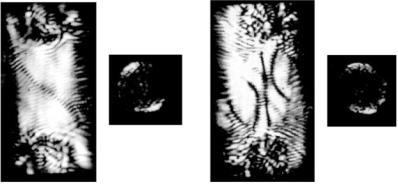
Figure 5.5 shows field distributions containing domains of tilted waves, as observed experimentally. Two domains (left) and four domains (right) are shown together with their corresponding far-field distributions. The directions of the waves traveling inside the domains correspond to the orientations of the spots in the far-field ring. The orientation drifted slowly with time, indicating that the orientation of the domains is independent of the boundaries both in the experiment and in the numerics. The domains are separated by vortex rows, as expected for domains of di erent flow.

86 5 Finite Detuning: Vortex Sheets and Vortex Lattices

Fig. 5.5. Domains of tilted waves separated by rows of vortices: near-field and far-field pictures. The resonator length was tuned to maintain the ring in the far field. Note the row of vortices separating the two domains of tilt in the snapshot at the left. Four domains of di erent tilt are visible in the right snapshot

In the experimental figure (Fig. 5.5) counterpropagating domains were recorded. In general, the directions of the TWs in neighboring domains can be at arbitrary angles. Di erent angles between domains result in di erent separations between vortices at the domain boundaries. Figure 5.6 illustrates boundaries between domains characterized by di erent angles of the TWs, from counterpropagating domains (Fig. 5.6a) to almost copropagating domains (Fig. 5.6d).

The counterpropagating domains in Fig. 5.6a were constructed from TWs with wavenumbers |k| = 5 × 2π, directed to the left in the middle of the figure, and to the right at the horizontal periodic boundary. The directions of the TWs can be seen clearly from the phase plots (right column). The vortex sheet contains 10 vortices over the integration range in this case of counterpropagating domains: the integral of the phase gradient over the corresponding closed loop is equal to 10 × 2π.

In general, the density of vortices in a vortex sheet is proportional to the projection of the di erence between the wavectors ∆k = k1 − k2 on the domain boundary; this can be shown by integration of the phase gradient of the field over a closed loop enclosing a unit length of the domain boundary.

The TW of the middle domain in Fig. 5.6b is directed upwards and to the left: it has the same modulus of the wavevector as in Fig. 5.6a (|k| = 5 × 2π), but has a horizontal component kx = −4×2π. The vortex sheet now contains 9 vortices, which can again be checked by the integration of the phase gradient over the corresponding closed loop.

The TW of the middle domain in Fig. 5.6c is directed upwards. The vortex sheet contains 5 vortices in this case. A peculiar feature is that, for the lower vortex sheet, the TWs “run apart” (in the vertical direction), and thus the vortices are ”stretched”. This domain boundary corresponds to a

5.3 Square Vortex Lattices

87

a)

b)

c)

d)

Fig. 5.6. TW domains, as obtained by numerical integration of (5.1). The parameters are ∆ = 2 and g = 1. Di erent initial conditions were used to generate di erent direction of the TW in the domain

source. The upper domain boundary, in contrast, represents a sink, since the corresponding TWs “run together”.

Finally, the domain boundaries in Fig. 5.6d contain only two vortices, since the TWs are almost copropagating: for the middle domain, kx = 2×2π. The bottom vortex sheet again corresponds to a line of sources, and the top vortex sheet corresponds to a line of sinks, which can be also seen from the size and shape of the vortices.

5.3 Square Vortex Lattices

Two counterpropagating TWs compete and do not result in a stable standingwave pattern, as shown in the previous section. Instead, they occupy di erent areas in space. However, four resonant TWs can coexist simultaneously, resulting in a stationary pattern,

A(r, t) =	j	(5.8)
	Aj exp(ikj r) .
	=1,4

The four wavevectors are directed as shown in Fig. 5.7. The pattern consists of two pairs of counterpropagating TWs, crossing at an angle of 90◦. Such cross-roll patterns have been found in lasers [2, 3] and in optical parametric oscillators [4].

By inserting (5.7) into (5.1) and neglecting the higher harmonics, we obtain the result that the amplitudes of the TW components of the square vortex lattice (SVL) are all equal to |Aj |2 = 1/5. The phases of the TWs obey the relation

Φ =	j	(5.9)
	ϕj = π .
	=1,4

88 5 Finite Detuning: Vortex Sheets and Vortex Lattices

Fig. 5.7. Square vortex lattice as obtained by numerical integration of (5.1): amplitude, phase and spatial Fourier spectrum of the field. The parameters are g = 0.4 and ∆ = 2. At the right, a schematic illustration of the four TWs forming the pattern is shown

A stability analysis based on the variational potential yields the result that the SVL corresponds to a local minimum in the parameter space of Aj [2]. Therefore the SVL is stable with respect to small perturbations. The tilted waves correspond to deeper minima of the potential, and standing waves, as discussed in the previous section, correspond to a saddle point.

In Fig. 5.8 the SVL is shown for a pump value significantly larger than that used in Fig. 5.7. Shocks between vortices are visible, as well as higher spatial harmonics in the spatial Fourier spectrum.

Fig. 5.8. Square vortex lattice as obtained by numerical integration of (5.1). The parameters are the same as in Fig. 5.7, except for the pump value, p = 9. Here, a version of (5.1) was used in which the pump parameter was normalized to p = 1, and the gain term (the first term on the right-hand side of (5.1)) contained the gain parameter explicitly

Two pairs of counterpropagating TWs can cross not only at an angle of 90◦, but also at arbitrary angles. Such angles lead to rhombic vortex lattices, as shown in Fig. 5.9. The picture resembles domains of counterpropagating TWs. Indeed, with increasing detuning, a rhombic vortex lattice becomes unstable and transforms into domains of counterpropagating TWs. The decay of a rhombic vortex lattice and the formation of TW domains is shown in Fig. 5.10.

5.3 Square Vortex Lattices

89

Fig. 5.9. Rhombic vortex lattice as obtained by numerical integration of (5.1). The parameters are the same as in Fig. 5.7. The lattice is constructed from four TWs with wavevectors kj = (±4×2π, ±2π); however, higher components in spatial Fourier spectrum appear

Fig. 5.10. Decay of a rhombic vortex lattice and formation of TW domains, as obtained by numerical integration of an unnormalized version of (5.1). The parameters are the same as in Fig. 5.9, except for the pump value, p = 4. The stationary distribution shown in Fig. 5.9 was taken as the initial condition for the calculation

Finally, we present experimental evidence of a square vortex lattice. Figure 5.11 shows the corresponding field distribution. The directions of the four tilted waves correspond to the orientations of the four spots in the far-field ring. The orientation of these spots drifted with time indicating that (1) not only a square but also a rhombic symmetry of the vortex lattice was possible, and (2) the symmetry of the pattern was independent of the boundaries.