9.4 Experiments

133

pump. In this case the soliton drifts towards the resonator axis, independently of its initial position and even without mirror tilting.

The most important characteristic that we require of the system, from the information-processing point of view, is the possibility of “writing” and “erasing” the solitons. This can be achieved by exploiting the characteristics of a resonator with spatially extended nonlinearities, which induces a strong competition between solitons, independent of their separation. In this case, a strong enough localized perturbation, externally injected into the system, can be used to create (or write) a new soliton at a desired location, which competes with another soliton previously existing at a di erent place, the latter soliton discriminated against (or erased) by the new one. This switching process is shown in Fig. 9.5.

Injection

Injection Fig. 9.5. The dynamics of switching of solitons by injection as obtained by numerical integration of (9.6) in the case of one spatial dimension. A first injection flash occurs at t = 40, and a second at t = 80. The peak amplitude of the first injection beam was 4.1, and that of the second beam was 4.4; the widths of the injection beams were the same in both cases

9.4 Experiments

All of the theoretical results presented in the previous sections have been experimentally reproduced. For the experiments, a self-imaging resonator configuration was used containing a photorefractive crystal as the amplifying medium, and a saturable absorber consisting of bacteriorhodopsin [6] or a dye cell. The amplifying medium and the absorber were placed either in the same place in the resonator (corresponding to model (9.2)) or in separate places (corresponding to model (9.6)). A schematic illustration of the experimental setup is shown in Fig. 9.6.

The saturation of the transmission of the intracavity saturable absorber was initiated by an additional (bleaching) unfocused beam controlled by a shutter.

134 9 Subcritical Solitons I: Saturable Absorber

Nd:YAG laser

SHG crystal

Dye cell

CCD Camera

BR absorber

to PC

He-Ne laser

Shutter

Fig. 9.6. Experimental setup used in the studies of solitons

We consider first some experiments with a PRO, located close to the absorber. Initially, the bleaching beam completely saturates the absorber, and the observed emission is a speckle structure, with optical vortices separated by shocks. When the bleaching beam is blocked, the absorber unsaturates and a domain structure develops, evolving into contracting stripes (the field density decreases with time). This experimental scenario is shown in Fig. 9.7, in good agreement with the numerical result (compare with Fig. 9.2).

(a)

(b)

(c)

(d)

Fig. 9.7. Experimentally observed evolution of the field after the bleaching beam is switched o . The time interval between successive plots is 10 s

When the pump intensity is increased, two-dimensional solitons can be stabilized, as discussed in the previous section. Depending on the pump value and, mainly, on the moment at which it is increased, a single soliton or a cluster of solitons can be stabilized. If the pump intensity is increased

9.4 Experiments

135

a)

b)

c)

d)

		Fig. 9.8. Stationary solitons and en-
		sembles of solitons, observed experi-
Near field	Far field	mentally in the near and far field of
		the resonator

relatively late, one or a few coexisting solitons are obtained (Figs. 9.8a,b). If the change is made earlier, larger soliton ensembles appear (Figs. 9.8c,d).

The properties of single solitons were studied experimentally with a dye laser in the near-field–far-field configuration. The dependence of the average laser output on the average pump power was measured experimentally, showing the bistability or hysteresis loop predicted by the theory (Fig. 9.9).

The transverse structure of the output field was also measured, at three characteristic pump values. For pump values in the bistability region, a quasiGaussian spatial soliton develops, as Fig. 9.9a shows. At the border between bistability and monostability, a super-Gaussian structure appears (Fig. 9.9b), while in the monostability domain a large-size structure with a strongly structured profile is observed (Fig. 9.9c). To create the soliton, the absorber cell was locally bleached for a short time. After the bleaching was removed, the soliton remained.

136 9 Subcritical Solitons I: Saturable Absorber

Transverse coordinate ( mm)

(a)

(b)

(c)

3

2

1

0

Pump power

Average LSA power ( mW )

0.12

(c)

0.10

0.08

(b)

0.06

0.04(a)

0.02

0.00

0

2

4

6

8

10

12

14

Average pump power ( mW)

Fig. 9.9. Experimentally measured hysteresis in the dependence of the laser output on the pump power, and the transverse structure of the output laser beam for three fixed pump powers: (a) small, quasi-Gaussian spatial soliton in the bistable region, (b) intermediate-size, super-Gaussian soliton at the border between bistability and monostability, and (c) large-size structure with a strongly structured profile in the monostable region

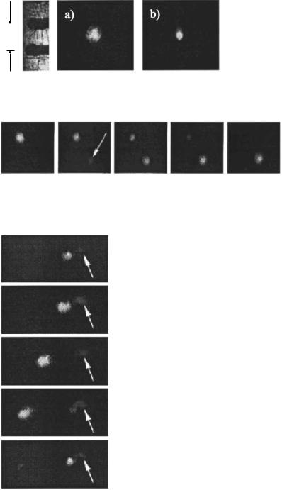
The size of the soliton depends on the di usion coe cient (note that, for small di raction, the di usion is nothing but a spatial scaling; see (9.4)), which, as discussed previously, is a function of the pump area. This dependence has been also observed in the experiments. As Fig. 9.10 shows, a focusing of the pump results in a broadening of the soliton.

The possibility of manipulating the solitons has been also demonstrated experimentally. Figure 9.11 shows the switching of a soliton. Once a soliton is “written” in a given place in the resonator cross section, the bleaching of the absorber at a di erent location results in the “erasing” of the first soliton and the creation of the new one.

Finally, the motion or drift of a soliton under the action of a phase gradient has been also tested. When one of the resonator mirrors is tilted, the soliton drifts at a constant velocity in the direction of the tilt (Fig. 9.12a). The

9.4 Experiments

137

1 mm

Fig. 9.10. Experimental observation of the spatial soliton structure in a laser: (a) for small pump area in the dye cell, and (b) for large pump area, illustrating the dependence of soliton size on di usion

Fig. 9.11. Switching of a soliton initiated by an external bleaching beam in a new position across the laser aperture. The arrow in the second picture indicates the place of incidence of the initiating beam. The time interval between neighboring pictures is 2.5 s

Fig. 9.12. The periodic soliton. Unidirectional drift motion and switching o occurs for a tilted resonator mirror when the bacteriorhodopsin absorber cell is subjected to permanent local bleaching by a laser beam