11.4 Phase Solitons

155

An expression for the velocity of the moving fronts in a potential system can also be derived. In the case of a cylindrically symmetric ring, the radial velocity v = dr0(t)/dt is [7]

∂F/∂r0

v = − , (11.16) 2π (∂A/∂r)2r dr

and is proportional to the force acting on the ring (the gradient of the variational potential) and inversely proportional to the “mass”, or inertia, of the ring. In the limit of large ring radius, the velocity can be evaluated analytically. In this case, using (11.14) for the potential, and evaluating the integral in the denominator in (11.16) in the same way as above, we obtain

2

2 + 3∆2

√

√

v =

−

6 − ∆2

5∆

,

(11.17)

−r

√

√

2

− 5∆

0

5

6 − ∆

that is, the velocity is inversely proportional to the ring radius.

The behavior of a circular domain boundary can be generalized to domains of arbitrary form. Assuming that the curvature of the dark line is su ciently small, the equation for the local motion of the curve is ∂R/∂t = −vc, where the local motion of the dark line is directed along its normal and is proportional to the local curvature c = ∂2R/∂l2, with the proportionality coe cient given by (11.17).

11.4 Phase Solitons

The above analysis predicts either the contraction or the expansion of domains. This conclusion is valid, however, only for a su ciently large radius of a domain or, equivalently, for a su ciently small curvature of a dark line. In other words, when diametrically opposite segments of the domain boundary do not interact. For small domains, when the diameter is of the same order of magnitude as the width of the domain boundary, the situation may be di erent. Indeed, numerical integration of the RSH equation sometimes shows that the dark rings stop contracting at some small radius. Figure 11.6 shows such a scenario, where an ensemble of stable dark rings of fixed radius evolves. We call these stationary small domains phase solitons, by analogy with the amplitude solitons studied in Chap. 9. A comparison of the profiles of the two types of solitons was shown in Figs. 8.1 and 8.7.

The variational approach of the previous section cannot predict analytically the existence of solitons, since the assumption r0/x0 1 is no longer valid. Numerical integration of (11.3), however, shows that phase solitons exist for detuning values in the range 0.287 ± 0.001 < ∆ < 0.460 ± 0.001.

The interaction of opposite segments of the ring results in a repulsive force that balances the attraction between the fronts due to the tendency to contraction, allowing soliton formation.

156 11 Phase Domains and Phase Solitons

Fig. 11.6. Evolution of phase domains obtained using the RSH equation for an intermediate signal detuning, ∆ = 0.35. Other parameters as in Fig. 11.3. The plots were obtained at times t = 0, 20, 150 and 1000

To demonstrate the repulsive e ect of the interaction, the potential (11.13) has been integrated numerically using the ansatz (11.12). Three characteristic plots are given in Fig. 11.7, showing the dependence of the potential on the radius of the ring for di erent values of the detuning ∆, together with the analytical approximation (11.14) (dashed lines).

As predicted from the 1D analytical calculations, for small detuning, the potential increases with the radius, leading to a contraction of the ring. Correspondingle, for large detuning, the potential decreases with increasing radius, leading to an expansion However, for some intermediate values of the detuning, the potential exhibits a minimum at some radius of the ring (the middle curve in Fig. 11.7; see also the inset). This potential minimum indicates the existence of phase solitons, with a radius corresponding to the potential minimum. The final distribution in the series shown in Fig. 11.6 is an ensemble of such solitons. These solitons are similar to those found in systems showing optical bistability, whose order parameter equation is also of Swift–Hohenberg type [9].

Although a variational analysis using the ansatz (11.12) yields a potential minimum at some radius of the dark ring, thereby predicting its stability, the evaluated stability range 0.39±0.01 < ∆ < 0.52±0.01 does not coincide with the numerically calculated stability range 0.287 ±0.001 < ∆ < 0.460 ±0.001.

F				∆=0.3
8
4				∆=0.45
0				∆=0.6
0	1	2	3	4	r0

Fig. 11.7. The potential obtained by evaluating (11.13) numerically with the ansatz (11.12), for a small detuning ∆ = 0.3, for a large detuning ∆ = 0.6 and for an intermediate value of detuning ∆ = 0.45. The 1D potentials calculated analytically (11.11) are shown by dashed lines. The case of ∆ = 0.45 is magnified in the inset

11.5 Nonmonotonically Decaying Fronts

157

The discrepancy between the numerically calculated soliton existence range and that obtained from the “monotonic” ansatz (11.12) suggests that some other mechanism is responsible for the stability of solitons. We consider next the nonmonotonic (oscillatory) spatial decay of the domain boundaries as a possible stabilizing mechanism.

11.5 Nonmonotonically Decaying Fronts

As can be seen from Fig. 11.8, numerical integration of the RSH equation in 1D indeed shows small amplitude oscillations in the decay of the fronts. The larger the detuning is, the larger is the spatial modulation of the tails of the domain boundaries.

	1	(a)	(b)	(c)
	0.5
A (x )	0	x	x	x
	- 0.5
	-1

Fig. 11.8. The order parameter A corresponding to a phase domain, as calculated from (11.3) in the 1D case, for di erent values of detuning. (a) ∆ = −0.75: domain boundaries are monotonic functions. (b) ∆ = 0: small spatial oscillations close to domain boundaries are visible. (c) ∆ = 0.75: strong spatial oscillations are

visible. The detuning value in the last case c) is close to the modulational-instability

√

threshold at ∆ = 2/3

Since the monotonic ansatz (11.6) in the form of a hyperbolic tangent does not describe these spatial oscillations correctly, an “oscillatory” ansatz must be used instead [10]. We use the ansatz

A(x) = sign(x) 1 − ∆2f(x) , (11.18)

where the profile function f, given by

f(x) = 1 − e−σ|x| cos(kx) ,

(11.19)

is characterized by a spatial decay rate σ and a spatial frequency k. In general, the ansatz (11.18) means that the domain boundaries decay with a complex-valued decay parameter Λ = σ+ik. The real part of Λ indicates the spatial decay of a perturbation, while the imaginary part indicates the spatial frequency of oscillation. These two unknown parameters can be found by minimizing the corresponding potential. Integration of (11.8) with the ansatz (11.18) gives a value for the potential which depends on the detuning ∆ and

158 11 Phase Domains and Phase Solitons

1.5
Λ			Im(Λ)
1.0
			Re(Λ)
0.5
0.0
-1.0	-0.5	0.0	0.5	∆

Fig. 11.9. The real and imaginary parts of the spatial decay rate Λ = σ+ik of a domain boundary, as a function of the detuning ∆

on the soliton parameters σ and k. The potential has a minimum corresponding to the correct values of σ and k. These values are given in Fig. 11.9 as a function of the detuning.

From Fig. 11.9, it follows that oscillatory behavior is more prominent for positive detuning, since σ < k. For negative detuning, σ > k, and the oscillations are relatively strongly damped, in accordance with Fig. 11.8. The dependence of the potential on the detuning is qualitatively the same as in Fig. 11.2, obtained with the monotonic ansatz. The di erence is only quantitative: the potential changes its sign from positive (domain contraction) to negative (domain expansion) at a detuning value ∆c ≈ 0.4616. Comparing this value with the numerically obtained value ∆c = 0.45 ± 0.05, we see that the results obtained from the nonmonotonic ansatz agree well with the numerically obtained results.

The nonmonotonic ansatz can be extended to 2D to analyze the stability of ring-shaped domain boundaries in 2D. In this case we take

A(r) = sign (r − r0) 1 − ∆2f(r − r0)f(r + r0) , (11.20)

where f is given by (11.19), r0 is the radius of the ring as in (11.12), and the decay parameters σ and k are taken from the results of the 1D variational study. The oscillatory ansatz and the numerically calculated soliton profile are compared in Fig. 11.10.

A calculation of the potential (11.8) using the ansatz (11.20) yields again a minimum at some ring radius, indicating the existence of solitons. This minimum exists in the detuning range 0.27 < ∆ < 0.46, which corresponds well to that obtained numerically, 0.287 ± 0.001 < ∆ < 0.460 ± 0.001. Again we note that the existence range calculated in the previous section by using the monotonic ansatz was very di erent from the existence range calculated numerically. Therefore one may conclude that a nonmonotonic decay of domain boundaries is essential for a correct description of solitons. The assumption of nonmonotonic decay allows one to calculate precisely the critical detuning value for contraction or expansion of domains, and also the existence range of localized solutions.

11.5 Nonmonotonically Decaying Fronts

159

A
0
- 1
x	r

Fig. 11.10. Left: profile of a dark line (kink) in 1D (solid line) and its approximation by the oscillatory ansatz (11.18) (dashed line), for ∆ = 0.3. Right: profile of a spatial soliton in 2D and its approximation by the ansatz (11.20), for ∆ = 0.4

Next we explore how, in general, the soliton stability range depends on the modulation of the tails. For this purpose, we assume that the dynamics of domain boundaries are described by the RSH equation, but that the modulation of the domain boundaries is enhanced (or reduced) by some additional (let us say, nonvariational) e ects [10]. This occurs, for example, in degenerate optical parametric oscillators (see Chap. 12). For this purpose, we keep the value of the k obtained from the variational analysis of the RSH equation (in which case k(∆) is a function only of the detuning), but allow arbitrary values of the decay parameter σ. The approach is somewhat artificial, but it allows one to understand qualitatively the role of the oscillatory fronts in the stabilization of solitons.

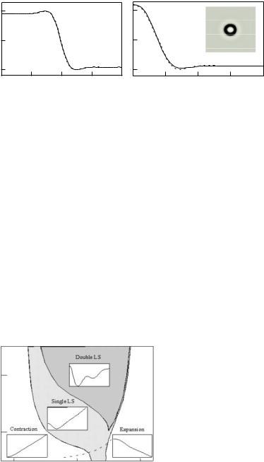
The resulting diagram is plotted in Fig. 11.11, which shows the soliton stability range in the plane (∆, 1/σ). The existence range grows with increasing oscillation of the decaying domain boundary (decreasing σ). The dashed curve corresponds to the decay rate calculated from the variational analysis of the RSH equation. The region above the dashed line corresponds to enhanced

4

σ–1

2

				Fig. 11.11. The soliton exis-
				tence range in the plane (∆, 1/σ),
				for a singleand a double-radius
	–1.0	0.0	1.0	ring soliton. The potentials cor-
				responding to di erent cases are
		∆
				shown in the insets

160 11 Phase Domains and Phase Solitons

spatial oscillations relative to the predictions of the RSH equation, and the region below the dashed line corresponds to reduced spatial oscillations.

For su ciently strong spatial oscillations, the soliton stability range may extend even the negative values of detuning. This is in good correspondence with results derived in the case of a DOPO, where a significant increase of the existence range is predicted (Chap. 12). Also, besides the fundamental soliton (a ring of minimum radius), higher-order solitons appear, characterized by

aset of discrete values of the ring radius r = nr0, where n = 1, 3, 5, ... and r0 is the radius of the fundamental soliton. The potential corresponding to

adouble-size ring soliton is shown in the inset. These higher-order solitons have been found numerically in a DOPO in [11] (see also Sect. 11.7).

The distributions in Fig. 11.12 show ensembles of solitons calculated from

amodel of a DOPO [2]. Besides the single-ring soliton, double-ring solitons are also possible here. Also, locked states of two single-ring solitons and even more complicated “molecules” were obtained.

Fig. 11.12. Ensembles of phase solitons in a DOPO. The parameters are E = 2, ω0 = 0, γ1 = γ0 = 1, a1 = 0.0005 and a0 = 0.00025. The integration was performed with periodic boundary conditions in a unit-size region. The signal detunings ω1, from left to right, are −0.3, −0.5, −0.6 and −0.6

11.6 Experimental Realization of Phase Domains

and Solitons

Although theoretical investigations of phase domains and solitons were initiated by studying the concrete example of a DOPO system, the first experiments on domains were performed with a degenerate four-wave mixer [12]. The equivalence of these two systems near the threshold was demonstrated theoretically in [5], on the basis of the common order parameter equation for both systems. Experimentally, the slow dynamics of the field in a DFWM based on a slow photorefractive material (BaTiO3) are very convenient for the observation of transients. The characteristic timescale of the system is about 1 s, which allows recording with ordinary video equipment.

The experimental scheme is shown in Fig. 11.13. Two counterpropagating pump beams (from a single-frequency Ar+ laser at 514.5 nm) illuminate

	11.6 Experimental Realization of Phase Domains and Solitons						161

Fig. 11.13. Schematic illustration of near-self-imaging resonator used for experiments to study phase domains and solitons. M, mirrors; f, focal length of lenses; l, deviation from self-imaging length; D, diaphragm, which filters the high transverse modes. The photorefractive crystal was pumped by two counterpropagating beams. This scheme is similar to that discussed in Chap. 9, but the pumping by two counterpropagating beams used here results in degenerate four-wave mixing

a photorefractive BaTiO3 crystal mounted inside a near-self-imaging linear resonator. In the limit of precise self-imaging, such a resonator has an infinite Fresnel number (within the limits of the paraxial approximation). All the transverse modes are exactly degenerate, allowing resonance for arbitrary images with complicated structure. Changing the resonator length with respect to the self-imaging length by l makes the resonator equivalent to a

plane-mirror resonator of length l. In the experiment l was 30 mm, which

√

corresponds to a characteristic spatial scale x0 = 100 m (∆x0 ≈ λl). Variation of the resonator length on the scale of an optical wavelength allowed us to vary the detuning parameter.

Typically, domains separated by black lines of irregular shape were observed in the emission. The domain boundaries can have quite complicated forms, including self-crossings, and in general they move. Figure 11.14 shows the intensity of a portion of the emitted radiation (left), and an interferogram made with a plane wave (right), showing a phase di erence of π between do-

Fig. 11.14. Snapshots of the field intensity (left) and interferogram (right). A phase shift of π between neighboring domains is visible in the interference picture

162 11 Phase Domains and Phase Solitons

Fig. 11.15. A contracting domain boundary for small resonator detuning. The domain boundary straightens, and the domains contract and disappear for such values of the detuning

Fig. 11.16. Expanding domains for large resonator detuning. The domains grow and a final labyrinth structure sets in

mains, thus proving the real-valued nature of the order parameter of the emitted field.

The dynamics of the domains depend strongly on the detuning, as follows from the theoretical treatment discussed above. For near-zero detuning a domain coarsening occurs. Experimental recordings in this regime are given in Fig. 11.15, showing the shrinking of a domain boundary (compare with Fig. 11.3). The domain boundaries finally disappear, and a homogeneous field results as the final state.

For moderately large detuning, the topology-preserving expansion of domain boundaries, as recorded experimentally, is shown in Fig. 11.16 (compare with Fig. 11.4). The domains expand until the whole space is filled, and a “labyrinth” pattern is reached as the final state.

The formation of solitons was also observed when the detuning was increased (Fig. 11.17). In the left plot a transient state is shown, in which some domains shrink and some domains have already shrunk to the minimum radius. In the plot at the right, a stationary state containing two solitons is shown.

In order to prove the stability of the solitons, the evolution of the length of a domain boundary was studied. In these experiments, a long domain boundary and one soliton were simultaneously present. As Fig. 11.18 shows, the long domain shrinks, whereas the soliton remains unchanged. The lengths