210 14 Patterns and Noise

This results in an exponent 1/2 of the Lorentz-like amplitude and phase power spectra.

Generalizing, the power spectrum of phase fluctuations for a D-dimensional systems (e.g. for a fractal-dimensional system) is of the form S−D(ω) ≈ ω−α where α = 2−D/2. For the amplitude fluctuations, one obtains a Lorentz-like power spectrum, saturating for low frequencies, and with an ω−α dependence for high frequencies. The width of the Lorentz-like power spectrum of amplitude fluctuations depends on the supercriticality parameter p: ω0 ≈ 2|p|.

14.1.2 Numerical Results

The spectral densities (14.8)–(14.12) calculated from the linearization were compared with densities obtained directly by numerical integration of the CGL equation (14.1) in one, two and three spatial dimensions. A CGL equation with real-valued coe cients b = c = 0 was numerically integrated with a supercriticality parameter p = 1.

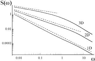
Temporal Power Spectra. The numerically calculated temporal power spectra are plotted in Fig. 14.1. The 1/ωα character of the noise spectra is most clearly seen in the case of a 1D system (here α = 3/2). In two dimensions the 1/ωα noise (α = 1) is visible over almost three decades of frequency, and in three dimensions (α = 1/2) over almost two decades. The dashed lines in Fig. 14.1 indicate the expected slopes.

Fig. 14.1. Total temporal power spectra of the noise in one, two and three spatial dimensions, as obtained by numerical integration of the CGL equation. The dashed lines show the slopes α = 1/2, α = 1 and α = 3/2. The spectra are arbitrary displaced vertically to distinguish between them. The integration period was t = 1000, and averaging was performed over 2500 realizations

The main obstacle to calculating the noise spectra numerically over the entire frequency range is the discretization of the spatial coordinates and of the

14.1 Noise in Condensates

211

time in the integration scheme. Discretization of space imposes a truncation of the higher spatial wavenumbers, and thus a ects the high-frequency components of the temporal spectra. Therefore, to obtain numerically the spectra over the entire frequency range, a series of separate calculations for di erent integration regions was performed, and the spectra in the corresponding frequency ranges were combined into one plot. The calculations shown Fig. 14.2

were performed for the 2D case with four di erent sizes of integration regions l = ln = 2π ×102.5−n/2 (n = 1, 2, 3, 4). The spectrum constructed by combin-

ing partially overlapping pieces results in a 1/ω dependence extending over more than five decades in frequency. A “kink” separating the low-frequency range (where the amplitude fluctuations are negligible compared with the phase fluctuations) and the high-frequency range (where the amplitude fluctuations are equal to the phase fluctuations) is visible in the power spectrum in Fig. 14.2a, and especially in the normalized power spectrum ωS(ω) in Fig. 14.2b.

Fig. 14.2. Total temporal power spectra of noise in 2D, as obtained by numerical integration of the CGL equation. The integration period was 107 temporal steps; averaging was performed over 2500 realizations. The calculations were performed with four di erent sizes of the integration region with di erent temporal steps

A multiscale numerical integration of the CGL equation in 1D and 3D was also performed. This showed the 1/ω3/2 and 1/ω1/2 dependences, respectively, over more than five decades of frequency (not shown).

212 14 Patterns and Noise

Spatial Power Spectra. Numerical discretization also distorts the spatial spectra, since it restricts the range of spatial wavenumbers. Therefore we also performed a series of calculations with di erent sizes of integration region, and combined the calculated averaged spatial spectra into one plot. The

results shown in Fig. 14.3 (2D case) were calculated with five di erent sizes of the integration region l = ln = 2π × 102.5−n/2 (n = 1, ..., 5). In this way

we obtained spectra by combining partially overlapping pieces, extending in total over around four decades.

Figure 14.3a shows the spectra on a log − log scale, where a 1/k2 character can be clearly seen, especially in the limits of long and short wavelengths. A “kink” at intermediate values of k, most clearly seen in Fig. 14.3b, joins spectra in the limits of long and short wavelengths which are both of the same slope but of di erent intensities.

One more reason to construct the spectra by combining pieces calculated separately is the finite size of the temporal step used in the split-step numerical technique. In order to obtain the correct spatial spectra in the longwavelength limit, a time-consuming integration is required. The long waves

Fig. 14.3. Total spatial power spectra of noise in two spatial dimensions, as obtained by numerical integration of the CGL equation. Averaging was performed over the time of the temporal steps. Each point corresponds to the averaged intensity of a discrete spatial mode. The calculations were performed with five di erent values of the size of the integration region, with di erent temporal steps. These spectra were combined into one plot. The dashed lines correspond to a 1/k2 dependence and are to guide the eye

14.1 Noise in Condensates

213

are very slow, the characteristic buildup time being of the order of τb ≈ 1/k2, as can be seen from (14.6) and (14.8), and this time diverges as k → 0. Thus one has to average for a very long time to obtain the correct statistics for the long waves. On the other hand, the characteristic buildup times for short wavelengths are very small, since the same relation τb ≈ 1/k2 holds. Here, correspondingly, in order to obtain the correct statistics of the mode occupation, one has to decrease the size of the temporal step as k → ∞. We thus come to the conclusion that one can never obtain the analytically predicted (correct) 1/k2 statistical distribution in a single numerical run with finite temporal steps (i.e. with a limited time resolution). A spectrum calculated with a fixed temporal step is shown in Fig. 14.4. In a log − log representation (Fig. 14.4a), a sharp decrease of the occupation of the large wavenumbers occurs. In a representation of the logarithm of the spectral density versus k2 (Fig. 14.4b), a straight line indicating an exponential decrease is obtained for large wavenumbers. The spectrum shown in Fig. 14.4, curiously enough, is thus precisely a Bose–Einstein distribution, which decays with a power law for long wavelengths, i.e. S(k → 0) k−2, and exponentially for short wavelengths, i.e. S(k → ∞) exp(k−2).

Fig. 14.4. The total spatial spectrum as obtained by numerical integration of the CGL equation in 1D for a fixed temporal step of ∆t = 0.05, but combined from four calculations with di erent sizes of integration region. Averaging was performed over a time t = 106 . Plot (a) shows the spectrum in a log −log representation, and the dashed line corresponds to a 1/k2 dependence, and (b) shows the spectrum in a single-log representation and the dashed line corresponds to an exp −k2 dependence

We note that the linear stability analysis does not lead to the Bose– Einstein distribution found numerically with finite temporal steps. The finite