3D Game Programming All In One (2004)

This page intentionally left blank

Team LRN

chapter 3

3D Programming

Concepts

In this chapter we will discuss how objects are described in their three dimensions in different 3D coordinate systems, as well as how we convert them for use in the 2D coordinate system of a computer display. There is some math involved here, but don't

worry—I'll do the heavy lifting.

We'll also cover the stages and some of the components of the rendering pipeline—a conceptual way of thinking of the steps involved in converting an abstract mathematical model of an object into a beautiful on-screen picture.

3D Concepts

In the real world around us, we perceive objects to have measurements in three directions, or dimensions. Typically we say they have height, width, and depth. When we want to represent an object on a computer screen, we need to account for the fact that the person viewing the object is limited to perceiving only two actual dimensions: height, from the top toward the bottom of the screen, and width, across the screen from left to right.

n o t e

Remember that we will be using the Torque Game Engine to do most of the rendering work involved in creating our game with this book. However, a solid understanding of the technology described in this section will help guide you in your decision-making later on when you will be designing and building your own models or writing code to manipulate those models in real time.

Therefore, it's necessary to simulate the third dimension, depth "into" the screen. We call this on-screen three-dimensional (3D) simulation of a real (or imagined) object a 3D

model. In order to make the model more visually realistic, we add visual characteristics,

89

Team LRN

90Chapter 3 ■ 3D Programming Concepts

such as shading, shadows, and textures. The entire process of calculating the appearance of the 3D model—converting it to an entity that can be drawn on a two-dimensional (2D) screen and then actually displaying the resulting image—is called rendering.

Coordinate Systems

When we refer to the dimensional measurement of an object, we use number groups called coordinates to mark each vertex (corner) of the object. We commonly use the variable names X, Y, and Z to represent each of the three dimensions in each coordinate group, or triplet. There are different ways to organize the meaning of the coordinates, known as coordinate systems.

We have to decide which of our variables will represent which dimension—height, width, or depth—and in what order we intend to reference them. Then we need to decide where the zero point is for these dimensions and what it means in relation to our object. Once we have done all that, we will have defined our coordinate system.

When we think about 3D objects, each of the directions is represented by an axis, the infinitely long line of a dimension that passes through the zero point. Width or left-right is usually the X-axis, height or up-down is usually the Y-axis, and depth or near-far is usually the Z-axis. Using these constructs, we have ourselves a nice tidy little XYZ-axis system, as shown in Figure 3.1.

						Now, when we consider a single
						object in isolation, the 3D space
						it occupies is called object space.
						The point in object space where
						X, Y, and Z are all 0 is normally
						the geometric center of an
						object. The geometric center of
						an object is usually inside the
						object. If positive X values are
						to the right, positive Y values
						are up, and positive Z values are
						away from you, then as you can
						see in Figure 3.2, the coordinate
Figure 3.1 XYZ-axis system.						system is called left-handed.

The Torque Game Engine uses a slightly different coordinate system, a right-handed one. In this system, with Y and Z oriented the same as we saw in the left-handed system, X is positive in the opposite direction. In what some people call Computer Graphics Aerobics, we can use the thumb, index finger, and middle finger of our hands to easily figure out the handedness of the system we are using (see Figure 3.3). Just remember that using this

Team LRN

3D Concepts

91

technique, the thumb is always the Y-axis, the index finger is the Z-axis, and the middle finger is the X-axis.

With Torque, we also orient the system in a slightly different way: The Z-axis is updown, the X-axis is somewhat left-right, and the Y-axis is somewhat near-far (see Figure 3.4). Actually, somewhat means that we specify left and right in terms of looking down on a map from above, with north at the top of the map. Right and left (positive and negative X) are east and west, respectively, and it follows that positive Y refers to north and negative Y to south. Don't forget that positive Z would be up, and negative Z would be down. This is a right-handed system that orients the axes to align with the way we would look at the world using a map from above. By specifying that the zero point for all three axes is a specific location on the map, and by using the coordinate system with the orientation just described, we have defined our world space.

Now that we have a coordinate system, we can specify any location on an object or in a world using a coordinate triplet, such as (5, 3, 2) (see Figure 3.5). By convention, this would be interpreted as X=5, Y= 3, Z= 2. A 3D triplet is always specified in XYZ format.

Figure 3.2 Left-handed coordinate system with vertical Y-axis.

Figure 3.3 Right-handed coordinate system with vertical Y-axis.

Take another peek at Figure 3.5. Notice anything? That's right—the Y-axis is vertical with the positive values above the 0, and the Z-axis positive side is toward us. It is still a right-handed coordinate system. The right-handed system with Y-up orientation is often used for modeling objects in isolation, and of course we call it object space, as described earlier. We are going to be working with this orientation and coordinate system for the next little while.

Team LRN

Figure 3.4 Right-handed coordinate system with vertical Z- axis depicting world space.

92

Chapter 3

■

3D Programming Concepts

3D Models

I had briefly touched on the idea that we can simulate, or model, any object by defining its shape in terms of its significant vertices (plural for vertex). Let's take a closer look, by starting with a simple 3D shape, or primitive—the cube—as depicted in Figure 3.6.

Figure 3.5 A point specified using an XYZ coordinate triplet.

Figure 3.6 Simple cube shown in a standard XYZ axis chart.

The cube's dimensions are two units wide by two units deep by two units high, or 2 2 2. In this draw-

ing, shown in object space, the geometric center is offset to a position outside the cube. I've done this in order to make it clearer what is happening in the drawing, despite my statement earlier that geometric centers are usually located inside an object. There are times when exceptions are not only possible, but necessary—as in this case.

Examining the drawing, we can see the object's shape and its dimensions quite clearly. The lower-left-front corner of the cube is located at the position where X=0, Y=1, and Z= 2. As an exercise, take some time to locate all of the other vertices (corners) of the cube, and note their coordinates.

If you haven't already noticed on your own, there is more information in the drawing than actually needed. Can you see how we can plot the coordinates by using the guidelines to find the positions on the axes of the vertices? But we can also see the actual coordinates of the vertices drawn right in the chart. We don't need to do both. The axis lines with their index tick marks and values really clutter up the drawing, so it has become somewhat accepted in computer graphics to not

Team LRN

3D Concepts

93

bother with these indices. Instead we try to use the minimum amount of information necessary to completely depict the object.

We only really need to state whether the object is in object space or world space and indicate the raw coordinates of each vertex. We should also connect the vertices with lines that indicate the edges.

If you take a look at Figure 3.7 you will see how easy it is to extract the sense of the shape, compared to the drawing in Figure 3.6. We specify which space definition we are using by the small XYZ-axis notation. The color code indicates the axis name, and the axis lines are drawn only for the positive directions. Different modeling tools use different color codes, but in this book dark yellow (shown as light gray) is the X-axis, dark cyan (medium gray) is the Y-axis, and dark magenta (dark gray) is the Z-axis. It is also common practice to place the XYZ-axis key at the geometric center of the model.

Figure 3.8 shows our cube with the geometric center placed where it reasonably belongs when dealing with an object in object space.

Now take a look at Figure 3.9. It is obviously somewhat more complex than our simple cube, but you are now armed with everything you need to know in order to understand it. It is a screen shot of a four-view drawing from the popular shareware modeling tool MilkShape 3D, in which a 3D model of a soccer ball was created.

In the figure, the vertices are marked with red

Figure 3.7 dots (which show as black in the picture), and axis key.

the edges are marked with light gray lines. The

axis keys are visible, although barely so in some views because they are obscured by the edge lines. Notice the grid lines that are used to help with aligning parts of the model. The three views with the gray background and grid lines are 2D construction views, while the fourth view, in the lowerright corner, is a 3D projection of the object. The upper-left view looks down from above, with the Y-axis in the vertical direction and the X-axis in the horizontal direction. The Z- axis in that view is not visible. The upper-right view is looking at the object from the front, with the Y-axis vertical

Simple cube with reduced XYZ-

Figure 3.8 Simple cube with axis key at geometric center.

Team LRN

94 Chapter 3 ■ 3D Programming Concepts

and the Z-axis horizontal; there is no X-axis. The lower-left view shows the Z-axis vertically and the X-axis horizontally with no Y-axis. In the lowerright view, the axis key is quite evident, as its lines protrude from the model.

3D Shapes

We've already encountered some of things that make up 3D models. Now it's time to round out that knowledge.

			As we've seen, vertices define
			the shape of a 3D model. We
Figure 3.9	Screen shot of sphere model.		connect the vertices with lines
			known as edges. If we connect
		three or more vertices with edges to create a closed figure,
		we've created a polygon. The simplest polygon is a trian-
		gle. In modern 3D accelerated graphics adapters, the
		hardware is designed to manipulate and display millions
		and millions of triangles in a second. Because of this
		capability in the adapters, we normally construct our
		models out of the simple triangle polygons instead of the
		more complex polygons, such as rectangles or pentagons
Figure 3.10	Polygons of	(see Figure 3.10).
varying complexity.		By happy coincidence, triangles are more than up to the
		task of modeling complex 3D shapes. Any complex poly-
		gon can be decomposed into a collection of triangles,
		commonly called a mesh (see Figure 3.11).

Figure 3.11 Polygons decomposed into triangle meshes.

The area of the model is known as the surface. The polygonal surfaces are called facets—or at least that is the traditional name. These days, they are more commonly called faces. Sometimes a surface can only be viewed from one side, so when you are looking at it from its "invisible" side, it's called a hidden surface, or hidden face. A double-sided face can be viewed from either side. The edges of hidden surfaces are called hidden lines. With

Team LRN

	Displaying 3D Models	95
most models, there are faces on the back side
of the model, facing away from us, called
backfaces (see Figure 3.12). As mentioned,
most of the time when we talk about faces in
game development, we are talking about tri-
angles, sometimes shortened to tris.

Displaying 3D Models

After we have defined a model of a 3D object of interest, we may want to display a view of it. The models are created in object space, but to

display them in the 3D world, we need to con-	Figure 3.12 The parts of a 3D shape.
vert them to world space coordinates. This

requires three conversion steps beyond the actual creation of the model in object space.

1.Convert to world space coordinates.

2.Convert to view coordinates.

3.Convert to screen coordinates.

Each of these conversions involves mathematical operations performed on the object's vertices.

The first step is accomplished by the process called transformation. Step 2 is what we call 3D rendering. Step 3 describes what is known as 2D rendering. First we will examine what the steps do for us, before getting into the gritty details.

Transformation

This first conversion, to world space coordinates, is necessary because we have to place our object somewhere! We call this conversion transformation. We will indicate where by applying transformations to the object: a scale operation (which controls the object's size), a rotation (which sets orientation), and a translation (which sets location).

World space transformations assume that the object starts with a transformation of (1.0,1.0,1.0) for scaling, (0,0,0) for rotation, and (0,0,0) for translation.

Every object in a 3D world can have its own 3D transformation values, often simply called transforms, that will be applied when the world is being prepared for rendering.

t i p

Other terms used for these kinds of XYZ coordinates in world space are Cartesian coordinates, or rectangular coordinates.

Team LRN

96

Chapter 3

■ 3D Programming Concepts

Scaling

We scale objects based upon a triplet

of scale factors where 1.0 indicates a

scale of 1:1.

The scale operation is written simi-

larly to the XYZ coordinates that are

used to denote the transformation,

except that the scale operation shows

Figure 3.13

Scaling.

how the size of the object has

changed. Values greater than 1.0 indi-

cate that the object will be made larger, and values less than 1.0 (but greater than 0) indicate that the object will shrink.

For example, 2.0 will double a given dimension, 0.5 will halve it, and a value of 1.0 means no change. Figure 3.13 shows a scale operation performed on a cube in object space. The original scale values are (1.0,1.0,1.0). After scaling, the cube is 1.6 times larger in all three dimensions, and the values are (1.6,1.6,1.6).

Rotation

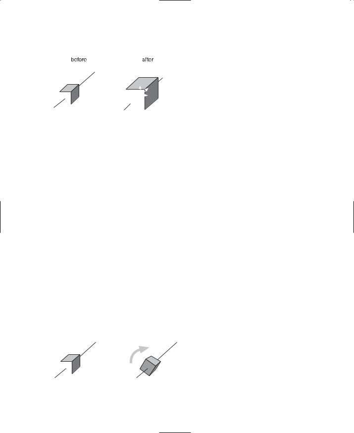
The rotation is written in the same way that XYZ coordinates are used to denote the transformation, except that the rotation shows how much the object is rotated around each of its three axes. In this book, rotations will be specified using a triplet of degrees as the unit of measure. In other contexts, radians might be the unit of measure used. There are also other methods of representing rotations that are used in more complex situations, but this is the way we'll do it in this book. Figure 3.14 depicts a cube being rotated by 30 degrees around the Y-axis in its object space.

It is important to realize that the order of the rotations applied to the object matters a great deal. The convention we will use is the roll-pitch-yaw method, adopted from the

aviation community. When we rotate the object, we roll it around its longitudinal (Z)
											axis. Then we pitch it around the
											lateral (X) axis. Finally, we yaw it
											around the vertical (Y) axis.
											Rotations on the object are applied
											in object space.
											If we apply the rotation in a differ-
											ent order, we can end up with a
											very different orientation, despite
											having done the rotations using the
Figure 3.14 Rotation.
											same values.

Team LRN

Displaying 3D Models

97

Translation

Translation is the simplest of the transformations and the first that is applied to the object

when transforming from object space to world space. Figure 3.15 shows a translation

operation performed on an object. Note that the vertical axis is dark gray. As I said earli-

er, in this book, dark gray represents the Z-axis. Try to figure out what coordinate system

we are using here. I'll tell you later in the chapter. To translate an object, we apply a vec-

tor to its position coordinates. Vectors can be specified in different ways, but the notation

we will use is the same as the XYZ triplet, called a vector triplet. For Figure 3.15, the vec-

tor triplet is (3,9,7). This indicates that the object will be moved three units in the posi-

tive X direction, nine units in the

positive Y direction, and seven

units in the positive Z direction.

Remember that this translation is

applied in world space, so the X

direction in this case would be east-

ward, and the Z direction would be

down (toward the ground, so to

speak). Neither the orientation nor

the size of the object is changed.

Figure 3.15 Translation.

Full Transformation

So now we roll all the operations together. We want to orient the cube a certain way, with a certain size, at a certain location. The transformations applied are scale (s)=1.6,1.6,1.6, followed by rotation (r)=0,30,0, and then finally translation (t)=3,9,7. Figure 3.16 shows the process.

Figure 3.16

Fully transforming the cube.

Team LRN