Baumol & Blinder MACROECONOMICS (11th ed)

LICENSED TO:

CHAPTER 4

Supply and Demand: An Initial Look

67

The Ups and Downs of Milk Consumption

The following excerpt from a U.S Department of Agriculture publication discusses some of the things that have affected the consumption of milk in the last century.

In 1909, Americans consumed a total of 34 gallons of fluid milk per person—27 gallons of whole milk and 7 gallons of milks lower in fat than whole milk, mostly buttermilk. . . . Fluid milk consumption shot up from 34 gallons per person in 1941 to a peak of 45 gallons per person in 1945. War production lifted Americans’ incomes but curbed civilian production and the goods consumers could buy. Many food items were rationed, including meats, butter and sugar. Milk was not rationed, and consumption soared. Since 1945, however, milk consumption has fallen steadily, reaching a record low of just under 23 gallons per person in 2001 (the latest year for which data are available). Steep declines in consumption of whole milk and buttermilk far outpaced an increase in other lower fat milks. By 2001, Americans were consuming less than 8 gallons per person of whole milk, compared with nearly 41 gallons in 1945 and 25 gallons in 1970. In contrast, per capita consumption of total lower fat milks was 15 gallons in 2001, up from 4 gallons in 1945 and 6 gallons

in 1970. These changes are consistent with increased public concern about cholesterol, saturated fat, and calories. However, decline in per capita consumption of fluid milk also may be attributed to competition from other beverages, especially carbonated soft drinks and bottled water, a smaller percentage of children and adolescents in the U.S., and a more ethnically diverse population whose diet does not normally include milk.

SOURCE: Judy Putnam and Jane Allshouse, “Trends in U.S. Per Capita Consumption of Dairy Products, 1909 to 2001,” Amber Waves: The Economics of Food, Farming, Natural Resources and Rural America, June 2003, U.S. Department of Agriculture, available at http://www.usda.gov.

Americans are switching to lower fat milks

person	40						Whole milk
	30
											Other lower fat milks
per
	20
Gallons
	10		Buttermilk
	0	1916	1923	1930	1937	1944	1951	1958	1965	1972	1979	1986	1993	2000
	1909

Lower fat milks include: buttermilk (1.5 percent fat), plain and flavored reduced fat milk (2 percent fat), low-fat milk (1 percent fat), nonfat milk, and yogurt made from these milks (except frozen yogurt).

Everything works in reverse if consumer incomes fall. Figure 8(b) depicts a leftward (inward) shift of the demand curve that results from a decline in consumer incomes. For example, the quantity demanded at the previous equilibrium price ($7.20) falls from 60 million pounds (point E) to 45 million pounds (point L on the demand curve D2D2). The initial price is now too high and must fall. The new equilibrium will eventually be established at point M, where the price is $7.10 and both quantity demanded and quantity supplied are 50 million pounds. In general:

Any influence that shifts the demand curve inward to the left, and that does not affect the supply curve, will lower both the equilibrium price and the equilibrium quantity.

SUPPLY SHIFTS AND SUPPLY-DEMAND EQUILIBRIUM

A story precisely analogous to that of the effects of a demand shift on equilibrium price and quantity applies to supply shifts. Figure 6 described the effects on the supply curve of beef if the number of farms increases. Figure 9(a) now adds a demand curve to the supply curves of Figure 6 so that we can see the supply-demand equilibrium. Notice that at the initial price of $7.20, the quantity supplied after the shift is 780 million pounds (point I on the supply curve S1S1), which is 30 percent more than the original quantity demanded of 600 million pounds (point E on the supply curve S0S0). We can see from the graph that the price of $7.20 is too high to be the equilibrium price; the price must fall. The new equilibrium point is J, where the price is $7.10 per pound and the quantity is 650 million pounds per year. In general:

Any change that shifts the supply curve outward to the right, and does not affect the demand curve, will lower the equilibrium price and raise the equilibrium quantity.

This must always be true if the industry’s demand curve has a negative slope, because the greater quantity supplied can be sold only if the price is decreased so as to induce customers to buy more.6 The cellular phone industry is a case in point. As more providers

6 Graphically, whenever a positively sloped curve shifts to the right, its intersection point with a negatively sloping curve must always move lower. Just try drawing it yourself.

Copyright 2009 Cengage Learning, Inc. All Rights Reserved. May not be copied, scanned, or duplicated, in whole or in part.

LICENSED TO:

68

PART 1

Getting Acquainted with Economics

FIGURE 9

Effects of Shifts of the Supply Curve

								S2
	D						D
				S0			V
per Pound					per Pound	$7.40		S0
	E		I	S1		U		E
Price	$7.20				Price	7.20
	7.10	J
	S0					S2
	S1					S0
			D					D
	60	65	78			37.5	50	60
	Quantity						Quantity
	(a)							(b)

have entered the industry, the cost of cellular service has plummeted. Some cellular carriers have even given away telephones as sign-up bonuses.

Figure 9(b) illustrates the opposite case: a contraction of the industry. The supply curve shifts inward to the left and equilibrium moves from point E to point V, where the price is $7.40 and quantity is 500 million pounds per year. In general:

Any influence that shifts the supply curve to the left, and does not affect the demand curve, will raise the equilibrium price and reduce the equilibrium quantity.

Many outside forces can disturb equilibrium in a market by shifting the demand curve or the supply curve, either temporarily or permanently. In 1998, for example, gasoline prices dropped because recession in Asia shifted the demand curve downward, as did a reduction in use of petroleum that resulted from a mild winter. In the summer of 1998, severely hot weather and lack of rain damaged the cotton crop in the United States, shifting the supply curve downward. Such outside influences change the equilibrium price and quantity. If you look again at Figures 8 and 9, you can see clearly that any event that causes either the demand curve or the supply curve to shift will also change the equilibrium price and quantity.

PUZZLE RESOLVED:

THOSE LEAPING OIL PRICES

The disturbing increases in the price of gasoline, and of the oil from which it is made, is attributable to large shifts in both demand and supply conditions. Americans are, for example, driving more and are buying gas-guzzling vehicles, and the resulting upward shift in the demand curve raises price. Instability in the Middle East and Russia has undermined supply, and that also raised prices. We have seen the results at the gas pumps. The following news-

paper story describes a sensational sort of change in supply conditions:

Aug. 10 (Bloomberg)—BP Plc and its partners in the Prudhoe Bay oil field in Alaska will spend about $170 million inspecting and repairing corroded pipelines that shut most of the production from the largest U.S. oil field.

Including costs to clean up and repair a line that leaked in March, the “rough estimate” rises to about $200 million, said Kemp Copeland, field manager for BP’s Prudhoe Bay operations. The figures include the cost of replacing 16 miles of feeder pipeline in the field.

The worst cost to BP will probably be the hit to its reputation, said Mark Gilman, an analyst at The Benchmark Company LLC in New York, who rates the shares “sell.”

Copyright 2009 Cengage Learning, Inc. All Rights Reserved. May not be copied, scanned, or duplicated, in whole or in part.

LICENSED TO:

CHAPTER 4

Supply and Demand: An Initial Look

69

“At some point this is going to prove very costly, as you’re going to be competing with folks whose reputation has not been subject to the same degree of punishment,” Gilman, who owns a “small” number of BP shares, said today in a phone interview.

The Prudhoe Bay shutdown is the latest blow for Chief Executive Officer John Browne, who faces a grand jury probe for an earlier Alaska spill, charges of market manipulation in the U.S. propane industry and fines from a Texas refinery blast that killed 15 workers. BP, which gets 40 percent of its sales from the U.S., last month said it will boost spending there to improve safety and maintenance.

London-based BP Plc said today it will know by the start of next week whether it can keep operating the western half of the field, which is currently producing as much as 137,000 barrels of oil a day. The entire field pumps 400,000 barrels a day, or 8 percent of U.S. output, when fully operational.

LOOKING FOR STEEL SUPPLIES

BP is asking suppliers U.S. Steel Corp. and Nippon Steel Corp. for faster delivery to a total of 51,000 feet of pipe it has already ordered for the repairs, BP Alaska President Steve Marshall said in conference call on Aug. 8. The pipe is scheduled to be delivered in October the earliest.

A supplier for another 30,000 feet of 24-inch pipe and 52,000 feet of 18-inch pipe is still needed, said Marshall.

BP, Houston-based ConocoPhillips and Exxon Mobil Corp. of Irving, Texas, are joint owners in the Prudhoe Bay field. ConocoPhillips, the third-largest U.S. oil company, earlier today declared force majeure on oil deliveries from Prudhoe Bay.

Force majeure allows companies to avoid penalties for failing to fulfill contracts because of unforeseen events. ConocoPhillips sells its Alaskan crude oil to refineries and brokers, according to spokesman Bill Tanner.

SOURCE: Ian McKinnon and Sonja Franklin, “BP Says Prudhoe Bay Repair Costs May Be $200 Million,” with reporting by Jim Kennett in Houston. Editor: Jordan (rsd)

Application: Who Really Pays That Tax?

Supply-and-demand analysis offers insights that may not be readily apparent. Here is an ex-

ample. Suppose your state legislature raises the gasoline tax by 10 cents per gallon. Service

station operators will then have to collect 10 additional

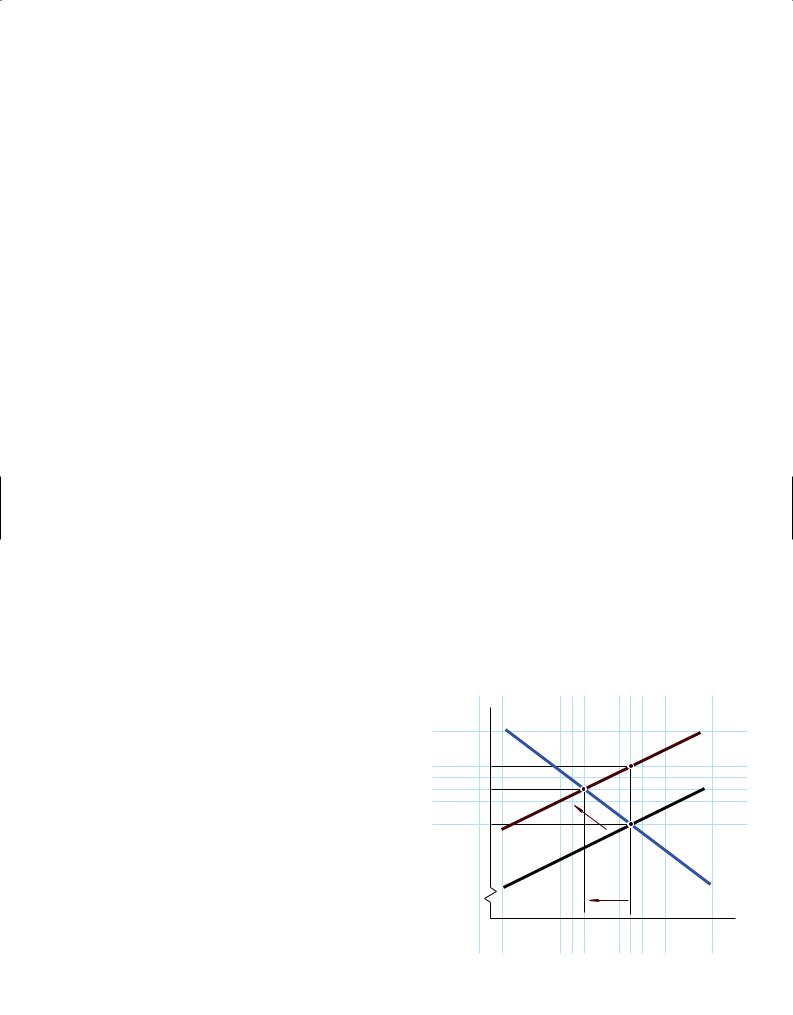
FIGURE 10

cents in taxes on every gallon they pump. They will con-

sider this higher tax as an addition to their costs and will

Who Pays for a New Tax on Products?

pass it on to you and other consumers by raising the

price of gas by 10 cents per gallon. Right? No, wrong—or

rather, partly wrong.

D

S1

The gas station owners would certainly like to pass on

the entire tax to buyers, but the market mechanism will

Gallon

$

2.64

M

allow them to shift only part of it—perhaps 6 cents per

E

1

S0

2.60

gallon. They will then be stuck with the remainder—

per

4 cents in our example. Figure 10, which is just another

supply-demand graph, shows why.

Price

2.54

The demand curve is the red curve DD. The supply

S1

E0

curve before the tax is the black curve S0S0. Before the

new tax, the equilibrium point is E0 and the price is

$2.54. We can interpret the supply curve as telling us at

D

what price sellers are willing to provide any given

S0

quantity. For example, they are willing to supply

Q2

Q1

30

50

quantity Q1 5 50 million gallons per year if the price is

Millions of

Gallons per

Year

$2.54 per gallon.

Copyright 2009 Cengage Learning, Inc. All Rights Reserved. May not be copied, scanned, or duplicated, in whole or in part.

LICENSED TO:

70

PART 1

Getting Acquainted with Economics

So what happens as a result of the new tax? Because they must now turn 10 cents per gallon over to the government, gas station owners will be willing to supply any given quantity only if they get 10 cents more per gallon than they did before. Therefore, to get them to supply quantity Q1 5 50 million gallons, a price of $2.54 per gallon will no longer suffice. Only a price of $2.64 per gallon will now induce them to supply 50 million gallons. Thus, at quantity Q1 5 50, the point on the supply curve will move up by 10 cents, from point E0 to point M. Because firms will insist on the same 10-cent price increase for any other quantity they supply, the entire supply curve will shift up by the 10-cent tax—from the black curve S0S0 to the new brick supply curve S1S1. And, as a result, the supply-demand equilibrium point will move from E0 to E1 and the price will increase from $2.54 to $2.60.

The supply curve shift may give the impression that gas station owners have succeeded in passing the entire 10-cent increase on to consumers—the distance from E0 to M—but look again. The equilibrium price has only gone up from $2.54 to $2.60. That is, the price has risen by only 6 cents, not by the full 10-cent amount of the tax. The gas station will have to absorb the remaining 4 cents of the tax.

Now this really looks as though we have pulled a fast one on you—a magician’s sleight of hand. After all, the supply curve has shifted upward by the full amount of the tax, and yet the resulting price increase has covered only part of the tax rise. However, a second look reveals that, like most apparent acts of magic, this one has a simple explanation. The explanation arises from the demand side of the supply-demand mechanism. The negative slope of the demand curve means that when prices rise, at least some consumers will reduce the quantity of gasoline they demand. That will force sellers to give up part of the price increase. In other words, firms must absorb the part of the tax—4 cents—that consumers are unwilling to pay. But note that the equilibrium quantity Q1 has fallen from 50 million gallons to Q2 5 30 million gallons—so both consumers and suppliers lose out in some sense.

This example is not an oddball case. Indeed, the result is almost always true. The cost of any increase in a tax on any commodity will usually be paid partly by the consumer and partly by the seller. This is so no matter whether the legislature says that it is imposing the tax on the sellers or on the buyers. Whichever way it is phrased, the economics are the same: The supply-demand mechanism ensures that the tax will be shared by both of the parties.

BATTLING THE INVISIBLE HAND: THE MARKET FIGHTS BACK

IDEAS FOR BEYOND THE FINAL EXAM

As we noted in our Ideas for Beyond the Final Exam in Chapter 1, lawmakers and rulers have often been dissatisfied with the outcomes of free markets. From Rome to Reno, and from biblical times to the space age, they have battled the invisible hand. Sometimes, rather than trying to adjust the workings of the market, governments have tried to raise or lower the prices of specific commodities by decree. In many such cases, the authorities felt that market prices were, in some sense, immorally low or immorally high. Penalties were therefore imposed on anyone offering the commodities in question at prices above or below those established by the authorities. Such legally imposed constraints on prices are called “price ceilings” and “price floors.” To see their result, we will focus on the use of price ceilings.

A price ceiling is a maximum that the price charged for a commodity cannot legally exceed.

Restraining the Market Mechanism: Price Ceilings

The market has proven itself a formidable foe that strongly resists attempts to get around its decisions. In case after case where legal price ceilings are imposed, virtually the same series of consequences ensues:

1.A persistent shortage develops because quantity demanded exceeds quantity supplied.

Queuing (people waiting in lines), direct rationing (with everyone getting a fixed allotment), or any of a variety of other devices, usually inefficient and unpleasant, must substitute for the distribution process provided by the price mechanism. Example: Rampant shortages in Eastern Europe and the former Soviet Union helped precipitate the revolts that ended communism.

Copyright 2009 Cengage Learning, Inc. All Rights Reserved. May not be copied, scanned, or duplicated, in whole or in part.

SOURCE: © AP Images/Angela Gaul

LICENSED TO:

CHAPTER 4

Supply and Demand: An Initial Look

71

P O L I C Y D E B AT E

ECONOMIC ASPECTS OF THE WAR ON DRUGS

For years now, the U.S. government has engaged in a highly publicized “war on drugs.” Billions of dollars have been spent on trying to stop illegal drugs at the country’s borders. In some sense, interdiction has succeeded: Federal agents have seized literally tons of cocaine and other drugs. Yet these efforts have made barely a dent in the flow of drugs to America’s city streets. Simple economic reasoning explains why.

When drug interdiction works, it shifts the supply curve of drugs to the left, thereby driving up street prices. But that, in turn, raises the rewards for potential smugglers and attracts more criminals into the “industry,” which shifts the supply curve back to the right. The net result is that increased shipments of drugs to U.S. shores replace much of what the authorities confiscate. This is why many economists believe that any successful antidrug program must concentrate on reducing demand, which would lower the street price of drugs, not on reducing supply, which can only raise it.

Some people suggest that the government should go even further and legalize many drugs. Although this idea remains a highly controversial position that few are ready to endorse, the reasoning behind it is straightforward. A stunningly high fraction of all the violent crimes committed in America— especially robberies and murders—are drug-

related. One major reason is that street prices of drugs are so high that addicts must steal to get the money, and drug traffickers are all too willing to kill to protect their highly profitable “businesses.”

How would things differ if drugs were legal? Because South American farmers earn pennies for drugs that sell for hundreds of dollars on the streets of Los Angeles and New York, we may safely assume that legalized drugs would be vastly cheaper. In fact, according to one estimate, a dose of cocaine would cost less than 50 cents. That, proponents point out, would reduce drug-related crimes dramatically. When, for example, was the last time you heard of a gang killing connected with the distribution of

cigarettes or alcoholic beverages?

The argument against legalization of drugs is largely moral: Should the state sanction potentially lethal substances? But there is an economic aspect to this position as well: The vastly lower street prices of drugs that would surely follow legalization would increase drug use. Thus, while legalization would almost certainly reduce crime, it may also produce more addicts. The key question here is, How many more addicts? (No one has a good answer.) If you think the increase in quantity demanded would be large, you are unlikely to find legalization an attractive option.

2.An illegal, or “black” market often arises to supply the commodity. Usually some individuals are willing to take the risks involved in meeting unsatisfied demands illegally. Example: Although most states ban the practice, ticket “scalping” (the sale of tickets at higher than regular prices) occurs at most popular sporting events and rock concerts.

3.The prices charged on illegal markets are almost certainly higher than those that would prevail in free markets. After all, lawbreakers expect some compensation for the risk of being caught and punished. Example: Illegal drugs are normally quite expensive. (See the accompanying Policy Debate box “Economic Aspects of the War on Drugs.”)

4.A substantial portion of the price falls into the hands of the illicit supplier instead of going to those who produce the good or perform the service. Example: A constant complaint during the public hearings that marked the history of theaterticket price controls in New York City was that the “ice” (the illegal excess charge) fell into the hands of ticket scalpers rather than going to those who invested in, produced, or acted in the play.

5.Investment in the industry generally dries up. Because price ceilings reduce the monetary returns that investors can legally earn, less money will be invested in industries that are subject to price controls. Even fear of impending price controls can have this effect. Example: Price controls on farm products in Zambia have prompted peasant farmers and large agricultural conglomerates alike to cut back production rather than grow crops at a loss. The result has been thousands of lost jobs and widespread food shortages.

Copyright 2009 Cengage Learning, Inc. All Rights Reserved. May not be copied, scanned, or duplicated, in whole or in part.

“If you leave me, you know, you’ll never see this kind of rent again.”

LICENSED TO:

72

PART 1

Getting Acquainted with Economics

FIGURE 11

Supply-Demand Diagram for Rental Housing

	D
Month	Market
Rent per	rent
	$2,000
	Rent
	ceiling
	1,200
	S
	0

Case Study: Rent Controls in New York City

These points and others are best illustrated by considering a concrete example involving price ceilings. New York is the only major city in the United States that has continuously legislated rent controls in much of its rental housing, since World War II. Rent controls, of course, are intended to protect the consumer from high rents. But most economists believe that rent control does not help the cities or their residents and that, in the long run, it leaves almost everyone worse off. Elementary supply-demand analysis shows us why.

Figure 11 is a supply-demand diagram for rental

units in New York. Curve DD is the demand curve and

S

curve SS is the supply curve. Without controls, equi-

librium would be at point E, where rents average

$2,000 per month and 3 million housing units are

occupied. If rent controls are effective, the ceiling price

E

must be below the equilibrium price of $2,000. But

with a low rent ceiling, such as $1,200, the quantity of

housing demanded will be 3.5 million units (point B),

C

B

whereas the quantity supplied will be only 2.5 million

D

units (point C).

The diagram shows a shortage of 1 million apart-

2.5

3

3.5

ments. This theoretical concept of a “shortage” mani-

Millions

of

Dwellings

fests itself in New York City as an abnormally low

Rented

per

Month

vacancy rate, that is, a low share of unoccupied apart-

ments available for rental—typically about half the

national urban average. Naturally, rent controls have spawned a lively black market in

New York. The black market raises the effective price of rent-controlled apartments in

many ways, including bribes, so-called key money paid to move up on a waiting list,

or the requirement that prospective tenants purchase worthless furniture at inflated

prices.

According to Figure 11, rent controls reduce the quantity supplied from 3 million to

2.5 million apartments. How does this reduction show up in New York? First, some prop-

erty owners, discouraged by the low rents, have converted apartment buildings into of-

fice space or other uses. Second, some apartments have been inadequately maintained.

After all, rent controls create a shortage, which makes even dilapidated apartments easy

to rent. Third, some landlords have actually abandoned their buildings rather than pay

rising tax and fuel bills. These abandoned buildings rapidly become eyesores and eventu-

ally pose threats to public health and safety.

An important implication of these last observations is that rent

controls—and price controls more generally—harm consumers in

ways that offset part or all of the benefits to those who are fortu-

nate enough to find and acquire at lower prices the product that

Cline

the reduced prices has made scarce. Tenants must undergo long

waits and undertake time-consuming searches to find an apart-

Richard

ment, the apartment they obtain is likely to be poorly main-

Collection, 1994

Rights Reserved.

tained or even decrepit, and normal landlord services are apt to

disappear. Thus, even for the lucky beneficiaries, rent control is

always far less of a bargain than the reduced monthly payments

make them appear to be. The same problems generally apply

YorkerNewThe©SOURCE:

Allcartoonbank.com.from

Part of the explanation is that most people simply do not un-

with other forms of price control as well.

With all of these problems, why does rent control persist in New York City? And why do other cities sometimes move in the same direction?

derstand the problems that rent controls create. Another part is that landlords are unpopular politically. But a third, and very

Copyright 2009 Cengage Learning, Inc. All Rights Reserved. May not be copied, scanned, or duplicated, in whole or in part.

LICENSED TO:

CHAPTER 4

Supply and Demand: An Initial Look

73

important, part of the explanation is that not everyone is hurt by rent controls—and those who benefit from controls fight hard to preserve them. In New York, for example, many tenants pay rents that are only a fraction of what their apartments would fetch on the open market. They are, naturally enough, quite happy with this situation. This last point illustrates another very general phenomenon:

Virtually every price ceiling or floor creates a class of people that benefits from the regulations. These people use their political influence to protect their gains by preserving the status quo, which is one reason why it is so difficult to eliminate price ceilings or floors.

Restraining the Market Mechanism: Price Floors

Interferences with the market mechanism are not always designed to keep prices low. Agricultural price supports and minimum wage laws are two notable examples in which the law keeps prices above free-market levels. Such price floors are typically accompanied by a standard series of symptoms:

1.A surplus develops as sellers cannot find enough buyers. Example: Surpluses of various agricultural products have been a persistent—and costly—problem for the U.S. government. The problem is even worse in the European Union (EU), where the common agricultural policy holds prices even higher. One source estimates that this policy accounts for half of all EU spending.7

2.Where goods, rather than services, are involved, the surplus creates a problem of disposal. Something must be done about the excess of quantity supplied over quantity demanded. Example: The U.S. government has often been forced to purchase, store, and then dispose of large amounts of surplus agricultural commodities.

3.To get around the regulations, sellers may offer discounts in disguised—and often un- wanted—forms. Example: Back when airline fares were regulated by the government, airlines offered more and better food and more stylishly uniformed flight attendants instead of lowering fares. Today, the food is worse, but tickets cost much less.

4.Regulations that keep prices artificially high encourage overinvestment in the industry. Even inefficient businesses whose high operating costs would doom them in an unrestricted market can survive beneath the shelter of a generous price floor. Example: This is why the airline and trucking industries both went through painful “shakeouts” of the weaker companies in the 1980s, after they were deregulated and allowed to charge market-determined prices.

Once again, a specific example is useful for understanding how price floors work.

A price floor is a legal minimum below which the price charged for a

commodity is not permitted to fall.

Case Study: Farm Price Supports and the Case of Sugar Prices

America’s extensive program of farm price supports began in 1933 as a “temporary method of dealing with an emergency”—in the years of the Great Depression, farmers were going broke in droves. These price supports are still with us today, even though farmers account for less than 2 percent of the U.S. workforce.8

One of the consequences of these price supports has been the creation of unsellable surpluses—more output of crops such as grains than consumers were willing to buy at the inflated prices yielded by the supports. Warehouses were filled to overflowing. New storage facilities had to be built, and the government was forced to set up programs in

7The Economist, February 20, 1999.

8Under major legislation passed in 1996, many agricultural price supports were supposed to be phased out over a seven-year period. In reality, many support programs, especially that for sugar, have changed little.

Copyright 2009 Cengage Learning, Inc. All Rights Reserved. May not be copied, scanned, or duplicated, in whole or in part.

LICENSED TO:

74

PART 1

Getting Acquainted with Economics

which grain from the unmanageable surpluses was shipped to poor foreign countries to combat malnutrition and starvation in those nations. Realistically, if price supports are to be effective in keeping prices above the equilibrium level, then someone must be prepared to purchase the surpluses that invariably result. Otherwise, those surpluses will somehow find their way into the market and drive down prices, undermining the price support program. In the United States (and elsewhere), the buyer of the surpluses has usually turned out to be the government, which makes its purchases at the expense of taxpayers who are forced to pay twice—once through taxes to finance the government purchases and a second time in the form of higher prices for the farm products bought by the American public.

One of the more controversial farm price supports involves the U.S. sugar industry. Sugar producers receive low-interest loans from the federal government and a guarantee that the price of sugar will not fall below a certain level.

In a market economy such as that found in the United States, Congress cannot simply set prices by decree; rather, it must take some action to enforce the price floor. In the case of sugar, that “something” is limiting both domestic production and foreign imports, thereby shifting the supply curve inward to the left. Figure 12 shows the mechanics involved in this price floor. Government policies shift the supply curve inward from S0S0 to S1S1 and drive the U.S. price up from 25¢ to 50¢ per pound. The more the supply curve shifts inward, the higher the price.

FIGURE 12

Supporting the Price

of Sugar

	S1
D	S 0
50¢
Price
25¢
S1
	D
	S 0
	Quantity

The sugar industry obviously benefits from the price-control program. But consumers pay for it in the form of higher prices for sugar and sugar-filled products such as soft drinks, candy bars, and cookies. Although estimates vary, the federal sugar price support program appears to cost consumers approximately $1.5 billion per year.

If all of this sounds a bit abstract to you, take a look at the ingredients in a U.S.-made soft drink. Instead of sugar, you will likely find “high-fructose corn syrup” listed as a sweetener. Foreign producers generally use sugar, but sugar is simply too expensive to be used for this purpose in the United States.

A Can of Worms

Our two case studies—rent controls and sugar price supports—illustrate some of the major side effects of price floors and ceilings but barely hint at others. Difficulties arise that

Copyright 2009 Cengage Learning, Inc. All Rights Reserved. May not be copied, scanned, or duplicated, in whole or in part.

LICENSED TO:

CHAPTER 4

Supply and Demand: An Initial Look

75

we have not even mentioned, for the market mechanism is a tough bird that imposes suitable retribution on those who seek to evade it by government decree. Here is a partial list of other problems that may arise when prices are controlled.

Favoritism and Corruption When price ceilings or floors create shortages or surpluses, someone must decide who gets to buy or sell the limited quantity that is available. This decision-making process can lead to discrimination along racial or religious lines, political favoritism, or corruption in government. For example, many prices were held at artificially low levels in the former Soviet Union, making queuing for certain goods quite common. Even so, Communist Party officials and other favored groups were somehow able to purchase the scarce commodities that others could not get.

Unenforceability Attempts to limit prices are almost certain to fail in industries with numerous suppliers, simply because the regulating agency must monitor the behavior of so many sellers. People will usually find ways to evade or violate the law, and something like the free-market price will generally reappear. But there is an important difference: Because the evasion process, whatever its form, will have some operating costs, those costs must be borne by someone. Normally, that someone is the consumer, who must pay higher prices to the suppliers for taking the risk of breaking the law.

Auxiliary Restrictions Fears that a system of price controls will break down invariably lead to regulations designed to shore up the shaky edifice. Consumers may be told when and from whom they are permitted to buy. The powers of the police and the courts may be used to prevent the entry of new suppliers. Occasionally, an intricate system of market subdivision is imposed, giving each class of firms a protected sphere in which others are not permitted to operate. For example, in New York City, there are laws banning conversion of rent-controlled apartments to condominiums.

Limitation of Volume of Transactions To the extent that controls succeed in affecting prices, they can be expected to reduce the volume of transactions. Curiously, this is true regardless of whether the regulated price is above or below the free-market equilibrium price. If it is set above the equilibrium price, the quantity demanded will be below the equilibrium quantity. On the other hand, if the imposed price is set below the freemarket level, the quantity supplied will be reduced. Because sales volume cannot exceed either the quantity supplied or the quantity demanded, a reduction in the volume of transactions is the result.9

Misallocation of Resources Departures from free-market prices are likely to result in misuse of the economy’s resources because the connection between production costs and prices is broken. For example, Russian farmers used to feed their farm animals bread instead of unprocessed grains because price ceilings kept the price of bread ludicrously low. In addition, just as more complex locks lead to more sophisticated burglary tools, more complex regulations lead to the use of yet more resources for their avoidance.

Economists put it this way: Free markets are capable of dealing efficiently with the three basic coordination tasks outlined in Chapter 3: deciding what to produce, how to produce it, and to whom the goods should be distributed. Price controls throw a monkey wrench into the market mechanism. Although the market is surely not flawless, and government interferences often have praiseworthy goals, good intentions are not enough. Any government that sets out to repair what it sees as a defect in the market mechanism runs the risk of causing even more serious damage elsewhere. As a prominent economist

9 See Discussion Question 4 at the end of this chapter.

Copyright 2009 Cengage Learning, Inc. All Rights Reserved. May not be copied, scanned, or duplicated, in whole or in part.

LICENSED TO:

76

PART 1

Getting Acquainted with Economics

once quipped, societies that are too willing to interfere with the operation of free markets soon find that the invisible hand is nowhere to be seen.

A SIMPLE BUT POWERFUL LESSON

Astonishing as it may seem, many people in authority do not understand the law of supply and demand, or they act as if it does not exist. For example, a few years ago the New York Times carried a dramatic front-page picture of the president of Kenya setting fire to a large pile of elephant tusks that had been confiscated from poachers. The accompanying story explained that the burning was intended as a symbolic act to persuade the world to halt the ivory trade.10 One may certainly doubt whether the burning really touched the hearts of criminal poachers, but one economic effect was clear: By reducing the supply of ivory on the world market, the burning of tusks forced up the price of ivory, which raised the illicit rewards reaped by those who slaughter elephants. That could only encourage more poaching—precisely the opposite of what the Kenyan government sought to accomplish.

| SUMMARY |

1.An attempt to use government regulations to force prices above or below their equilibrium levels is likely to lead to shortages or surpluses, to black markets in which goods are sold at illegal prices, and to a variety of other problems. The market always strikes back at attempts to repeal the law of supply and demand.

2.The quantity of a product that is demanded is not a fixed number. Rather, quantity demanded depends on such influences as the price of the product, consumer incomes, and the prices of other products.

3.The relationship between quantity demanded and price, holding all other things constant, can be displayed graphically on a demand curve.

4.For most products, the higher the price, the lower the quantity demanded. As a result, the demand curve usually has a negative slope.

5.The quantity of a product that is supplied depends on its price and many other influences. A supply curve is a graphical representation of the relationship between quantity supplied and price, holding all other influences constant.

6.For most products, supply curves have positive slopes, meaning that higher prices lead to supply of greater quantities.

7.A change in quantity demanded that is caused by a change in the price of the good is represented by a movement along a fixed demand curve. A change in

quantity demanded that is caused by a change in any other determinant of quantity demanded is represented by a shift of the demand curve.

8.This same distinction applies to the supply curve: Changes in price lead to movements along a fixed supply curve; changes in other determinants of quantity supplied lead to shifts of the entire supply curve.

9.A market is said to be in equilibrium when quantity supplied is equal to quantity demanded. The equilibrium price and quantity are shown by the point on the supply-demand graph where the supply and demand curves intersect. The law of supply and demand states that price and quantity tend to gravitate to this point in a free market.

10.Changes in consumer incomes, tastes, technology, prices of competing products, and many other influences lead to shifts in either the demand curve or the supply curve and produce changes in price and quantity that can be determined from supply-demand diagrams.

11.A tax on a good generally leads to a rise in the price at which the taxed product is sold. The rise in price is generally less than the tax, so consumers usually pay less than the entire tax.

12.Consumers generally pay only part of a tax because the resulting rise in price leads them to buy less and the cut in the quantity they demand helps to force price down.

10 The New York Times, July 19, 1989.

Copyright 2009 Cengage Learning, Inc. All Rights Reserved. May not be copied, scanned, or duplicated, in whole or in part.