Baumol & Blinder MACROECONOMICS (11th ed)

SOURCE: © Popperfoto/Getty Images

LICENSED TO:

CHAPTER 6

The Goals of Macroeconomic Policy

107

The Wonders of Compound Interest

Growth rates, like interest rates, compound so that, for example, 10 years of growth at 3 percent per year leaves the economy more than 30 percent larger. How much more? The answer is 34.4 percent. To see how we get this figure, start with the fact that $100 left in a bank account for one year at 3 percent interest grows to $103, which is 1.03 3 $100. If left for a second year, that $103 will grow another 3 percent—to 1.03 3 $103 5 $106.09, which is already more than $106. Compounding has begun.

Notice that 1.03 3 $103 is (1.03)2 3 $100.

Similarly, after three years the original $100 will grow to (1.03)3 3 $100 5 $109.27. As you can see, each additional year adds another 1.03 growth factor to the multiplication. Now returning to answer our original question, after 10 years of compounding, the depositor will have (1.03)10 3 $100 5 $134.39 in the bank. Thus the balance will have grown by 34.4 percent. By identical logic, an economy growing at 3 percent per year for 10 years will expand 34.4 percent in total.

You may not be impressed by the difference between 30 percent and 34.4 percent. If so, follow the logic for longer periods. After 20 years of 3 percent growth, the economy will be 80.6 percent bigger (because (1.03)20 5 1.806), not just 60 percent bigger. After 50 years, cumulative growth will be 338 percent, not 150 percent. And after a century, it will be 1,822 percent, not just 300 percent. Now we are talking about large discrepancies! No wonder Einstein once said, presumably in jest, that compounding was the most powerful force in the universe.

The arithmetic of growth leads to a convenient “doubling rule” that you can do in your head. If something (the money in a bank account, the GDP of a country, and so on) grows at an annual rate of g percent, how long will it take to double? The approximate answer is 70/g, so the rule is often called “the Rule of 70.” For example, at a 2 percent growth rate, something doubles in about 70/2 5 35 years. At a 3 percent growth rate, doubling takes roughly 70/3 5 23.33 years. Yes, small differences in growth rates can make a large difference.

Now fast-forward more than a century. By 1979, the United States had become the world’s preeminent economic power, Japan had emerged as the clear number two, and the United Kingdom had retreated into the second rank of nations. Obviously, the Japanese economy grew faster than the U.S. economy during this century, while the British economy grew more slowly, or else this stunning transformation of relative positions would not have occurred. But the magnitudes of the differences in growth rates may astound you.

Over the 109-year period, GDP per capita in the United States grew at a 2.3 percent compound annual rate while the United Kingdom’s growth rate was 1.8 percent—a difference of merely 0.5 percent per annum, but compounded for more than a century. And what of Japan? What growth rate propelled it from obscurity into the front rank of nations? The answer is just 3.0 percent, a mere 0.7 percent per year faster than the United States. These numbers show vividly what a huge difference a 0.5 or 0.7 percentage point change in the growth rate makes, if sustained for a long time.

Economists define the productivity of a country’s labor force (or “labor productivity“) as the amount of output a typical worker turns out in an hour of work. For example, if output is measured by GDP, productivity would be measured by GDP divided by the total number of hours of work. It is the growth rate of productivity that determines whether living standards will rise rapidly or slowly.

PRODUCTIVITY GROWTH IS (ALMOST) EVERYTHING IN THE LONG RUN As we pointed out in our list of Ideas for Beyond the Final Exam, only rising productivity can raise standards of living in the long run. Over long periods of time, small differences in rates of productivity growth compound like interest in a bank account and can make an enormous difference to a society’s prosperity. Nothing contributes more to material wellbeing, to the reduction of poverty, to increases in leisure time, and to a country’s ability to finance education, public health, environmental improvement, and the arts than its productivity growth rate.

Labor productivity is the amount of output a worker turns out in an hour (or a week, or a year) of labor. If output is measured by GDP, it is GDP per hour of work.

IDEAS FOR

BEYOND THE

FINAL EXAM

Copyright 2009 Cengage Learning, Inc. All Rights Reserved. May not be copied, scanned, or duplicated, in whole or in part.

LICENSED TO:
108	PART 2 The Macroeconomy: Aggregate Supply and Demand
		ISSUE:		IS FASTER GROWTH ALWAYS BETTER?

How fast should the U.S. economy, or any economy, grow? At first, the question may seem silly. Isn’t it obvious that we should grow as fast as possible? After all, that will make us all richer. In a broad sense, economists agree; faster growth is generally preferred to slower growth. But as we shall see in a few pages, further thought suggests that the apparently naive question is not quite as silly as it sounds. Growth comes at a cost. So more may not always be better.

THE CAPACITY TO PRODUCE: POTENTIAL GDP

AND THE PRODUCTION FUNCTION

Potential GDP is the real GDP that the economy would produce if its labor and other resources were fully employed.

The labor force is the number of people holding or seeking jobs.

The economy’s production function shows the volume of output that can be produced from given inputs (such as labor and capital), given the available technology.

FIGURE 1

The Economy’s

Production Function

Questions like how fast our economy can or should grow require quantitative answers. Economists have invented the concept of potential GDP to measure the economy’s normal capacity to produce goods and services. Specifically, potential GDP is the real gross domestic product (GDP) an economy could produce if its labor force was fully employed.

Note the use of the word normal in describing capacity. Just as it is possible to push a factory beyond its normal operating rate (by, for example, adding a night shift), it is possible to push an economy beyond its normal full-employment level by working it very hard. For example, we observed in the last chapter that the unemployment rate dropped as low as 1.2 percent under abnormal conditions during World War II. So when we talk about employing the labor force fully, we do not mean a measured unemployment rate of zero.

Conceptually, we estimate potential GDP in two steps. First, we count up the available supplies of labor, capital, and other productive resources. Then we estimate how much output these inputs could produce if they were all fully utilized. This second step—the transformation of inputs into outputs—involves an assessment of the economy’s technology. The more technologically advanced an economy, the more output it will be able to produce from any given bundle of inputs—as we emphasized in Chapter 3’s discussion of the production possibilities frontier.

To help us understand how technology affects the relationship between inputs and outputs, it is useful to introduce a tool called the production function—which is simply a mathematical or graphical depiction of the relationship between inputs and outputs. We will use a graph in our discussion.

For a given level of technology, Figure 1 shows how output (measured by real GDP on the vertical axis) depends on labor input (measured by hours of work on the horizontal

			M
	GDP	Y1
		A	K
	Real
		Y0

0	L0 Labor input
	(hours)

(a) Effect of better technology

		B	K1
		Y1
	GDP	A
	Real		K0
		Y0

0 L0 Labor input (hours)

(b) Effect of more capital

SOURCE: Bureau of Labor Statistics. Data pertain to the nonfarm business sector.

Copyright 2009 Cengage Learning, Inc. All Rights Reserved. May not be copied, scanned, or duplicated, in whole or in part.

LICENSED TO:

CHAPTER 6

The Goals of Macroeconomic Policy

109

axis). To read these graphs, and to relate them to the concept of potential GDP, begin with the black curve OK in Figure 1(a), which shows how GDP depends on labor input, holding both capital and technology constant. Naturally, output rises as labor inputs increase as we move outward along the curve OK, just as you would expect. If the country’s labor force can supply L0 hours of work when it is fully employed, then potential GDP is Y0 (see point A). If the technology improves, the production function will shift upward—say, to the brickcolored curve labeled OM—meaning that the same amount of labor input will now produce more output. The graph shows that potential GDP increases to Y1.

Now what about capital? Figure 1(b) shows two production functions. The black curve OK0 applies when the economy has some lower capital stock, K0. The higher, brick-colored curve OK1 applies when the capital stock is some higher number, K1. Thus, the production function tells us that potential GDP will be Y0 if the capital stock is K0 (see point A) but Y1 if the capital stock is K1 instead (see point B). Once again, this relationship is just what you would expect: The economy can produce more output with the same amount of labor if workers have more capital to work with.

You can hardly avoid noticing the similarities between the two panels of Figure 1: Better technology, as in Figure 1(a), or more capital, as in Figure 1(b), affect the production function in more or less the same way. In general:

Either more capital or better technology will shift the production function upward and therefore raise potential GDP.

THE GROWTH RATE OF POTENTIAL GDP

With this new tool, it is but a short jump to potential growth rates. If the size of potential GDP depends on the size of the economy’s labor force, the amount of capital and other resources it has, and its technology, it follows that the growth rate of potential GDP must depend on

•The growth rate of the labor force

•The growth rate of the nation’s capital stock

•The rate of technical progress

To sharpen the point, observe that real GDP is, by definition, the product of the total hours of work in the economy times the amount of output produced per hour—what we have just called labor productivity:

GDP 5 Hours of work 3 Output per hour 5 Hours of work 3 Labor productivity.

For example, in the United States today, in round numbers, GDP is about $14 trillion and total hours of work per year are about 250 billion. Thus labor productivity is roughly $14 trillion/250 billion hours 5 $56 per hour.

How fast can the economy increase its productive capacity? By transforming the preceding equation into growth rates, we have our answer: The growth rate of potential GDP is the sum of the growth rates of labor input (hours of work) and labor productivity:1

Growth rate of potential GDP 5 Growth rate of labor input 1 Growth rate of labor productivity

In the United States in recent years, labor input has been increasing at a rate of about 1 percent per year. But labor productivity growth, which was very slow until the mid1990s, has leaped upward since then—averaging about 2.6 percent per annum from 1995 to 2007. Together, these two figures imply an estimated growth rate of potential GDP in the 3.6 percent range over the past dozen years.

1 You may be wondering about what happened to capital. The answer, as we have just seen in our discussion of the production function, is that one of the main determinants of potential GDP, and thus of labor productivity, is the amount of capital that each worker has to work with. Accordingly, the role of capital is incorporated into the productivity number, that is, the growth rate of labor productivity depends on the growth rate of capital.

Copyright 2009 Cengage Learning, Inc. All Rights Reserved. May not be copied, scanned, or duplicated, in whole or in part.

LICENSED TO:

110

PART 2

The Macroeconomy: Aggregate Supply and Demand

TABLE 1

Recent Growth Rates of Real

GDP in the United States

	Growth Rate
Years	per Year

Do the growth rates of potential GDP and actual GDP match up? The answer is an important one to which we will return often in this book:

Over long periods of time, the growth rates of actual and potential GDP are normally quite similar. But the two often diverge sharply over short periods owing to cyclical fluctuations.

	1995–1997	4.1%			Table 1 illustrates this point with some recent U.S. data. Since 1994, GDP growth
	1997–1999	4.3
					rates over two-year periods have ranged from as low as 2.1 percent per annum to as
	1999–2001	2.2
					high as 4.3 percent. Over the entire 12-year period, GDP growth averaged 3.1 per-
	2001–2003	2.1
					cent, which is probably just a bit above current estimates of the growth rate of
	2003–2005	3.4
	2005–2007	2.5			potential GDP.
	1995–2007	3.1			The next chapter is devoted to studying the determinants of economic growth and
					some policies that might speed it up. But we already know from the production func-
SOURCE: U.S. Department of Commerce.
					tion that there are two basic ways to boost a nation’s growth rate—other than faster
			population growth and simply working harder. One is accumulating more capital. Other
			things being equal, a nation that builds more capital for its future will grow faster. The
			other way is by improving technology. When technological breakthroughs are coming at a
			fast and furious pace, an economy will grow more rapidly. We will discuss both of these
			factors in detail in the next chapter. First, however, we need to address the more basic
			question posed earlier in this chapter.

ISSUE REVISITED: IS FASTER GROWTH ALWAYS BETTER?

It might seem that the answer to this question is obviously yes. After all, faster growth of either labor productivity or GDP per person is the route to higher living standards. But exceptions have been noted.

For openers, some social critics have questioned the desirability of faster economic growth as an end in itself, at least in the rich countries. Faster growth brings more wealth, and to most people the desirability of wealth is

beyond question. “I’ve been rich and I’ve been poor. Believe me, honey, rich is better,” singer Sophie Tucker once told an interviewer. And most people seem to share her sentiment. To those who hold this belief, a healthy economy is one that produces vast quantities of jeans, pizzas, cars, and computers.

Yet the desirability of further economic growth for a society that is already quite wealthy has been questioned on several grounds. Environmentalists worry that the sheer increase in the volume of goods imposes enormous costs on society in the form of crowding, pollution, global climate change, and proliferation of wastes that need disposal. It has, they argue, dotted our roadsides with junkyards, filled our air with pollution, and poisoned our food with dangerous chemicals.

Some psychologists and social critics argue that the never-ending drive for more and better goods has failed to make people happier. Instead, industrial progress has transformed the satisfying and creative tasks of the artisan into the mechanical and dehumanizing routine of the assembly-line worker. In the United States, it even seems to be driving people to work longer and longer hours. The question is whether the vast outpouring of material goods is worth all the stress and environmental damage. In fact, surveys of self-reported happiness show that residents of richer countries are no happier, on average, than residents of poorer countries.

But despite this, most economists continue to believe that more growth is better than less. For one thing, slower growth would make it extremely difficult to finance programs that improve the quality of life—including efforts to protect the environment. Such programs are costly, and the evidence suggests that people are willing to pay for them only after their incomes reach a certain level. Second, it would be difficult to prevent further economic growth even if we were so inclined. Mandatory controls are abhorrent to most Americans; we cannot order people to stop being inventive and hardworking. Third, slower economic growth would seriously hamper efforts to

Copyright 2009 Cengage Learning, Inc. All Rights Reserved. May not be copied, scanned, or duplicated, in whole or in part.

LICENSED TO:

CHAPTER 6

The Goals of Macroeconomic Policy

111

eliminate poverty—both within our own country and throughout the world. Much of the earth’s population still lives in a state of extreme want. These unfortunate people are far less interested in clean air and fulfillment in the workplace than they are in more food, better clothing, and sturdier shelters.

All that said, economists concede that faster growth is not always better. One important reason will occupy our attention later in Parts 2 and 3: An economy that grows too fast may generate inflation. Why? You were introduced to the answer at the end of the last chapter: Inflation rises when aggregate demand races ahead of aggregate supply. In plain English, an economy will become inflationary when people’s demands for goods and services expand faster than its capacity to produce them. So we probably do not want to grow faster than the growth rate of potential GDP, at least not for long.

Should society then seek the maximum possible growth rate of potential GDP? Maybe, but maybe not. After all, more rapid growth does not come for free. We have noted that building more capital is one good way to speed the growth of potential GDP. But the resources used to manufacture jet engines and computer servers could be used to make home air conditioners and video games instead. Building more capital imposes an obvious cost on a society: The citizens must consume less today. Saying this does not argue against investing for the future. Indeed, most economists believe we need to do more of that. But we must realize that faster growth through capital formation comes at a cost—an opportunity cost. Here, as elsewhere, you don’t get something for nothing.

PART 2: THE GOAL OF LOW UNEMPLOYMENT

We noted earlier that actual GDP growth can differ sharply from potential GDP growth over periods as long as several years. These macroeconomic fluctuations have major implications for employment and unemployment. In particular:

When the economy grows more slowly than its potential, it fails to generate enough new
jobs for its ever-growing labor force. Hence, the unemployment rate rises. Conversely,	The unemployment rate
GDP growth faster than the economy’s potential leads to a falling unemployment rate.	is the number of unem-
High unemployment is socially wasteful. When the economy does not create enough	ployed people, expressed as
	a percentage of the labor
jobs to employ everyone who is willing to work, a valuable resource is lost. Potential	force.
goods and services that might have been produced and enjoyed by consumers are lost for-
ever. This lost output is the central economic cost of high unemployment, and we can
measure it by comparing actual and potential GDP.
That cost is considerable. Table 2 summarizes the idleness of workers and machines,
and the resulting loss of national output, for some of the years of lowest economic activity
in recent decades. The second column lists the civilian unemployment rate and thus meas-
ures unused labor resources. The third lists the percentage of industrial capacity that

	U.S. manufacturers were actually using, which indicates the extent to
	which plant and equipment went unused. The fourth column esti-
	mates the shortfall between potential and actual real GDP. We see that	TABLE 2
	unemployment has cost the people of the United States as much as an	The Economic Costs of High Unemployment
	8.1 percent reduction in their real incomes.
			Civilian	Capacity		Real GDP Lost
	Although Table 2 shows extreme examples, our inability to utilize
			Unemployment	Utilization		Due to Idle
	all of the nation’s available resources was a persistent economic prob-	Year	Rate		Rate	Resources
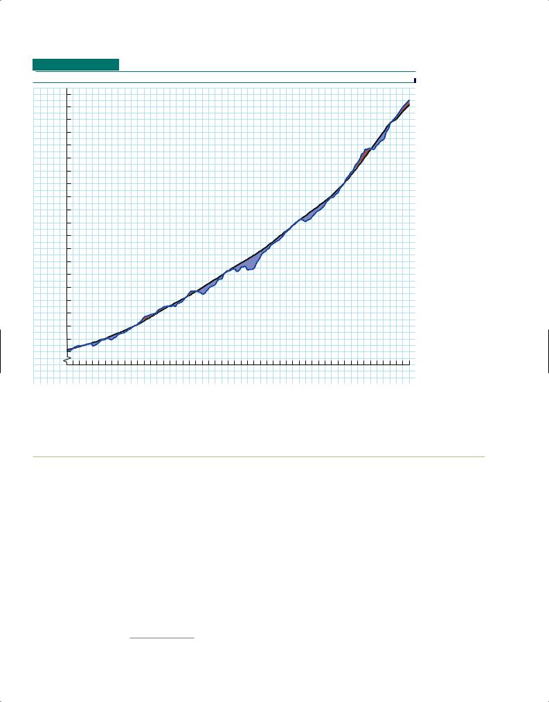
	lem for decades. The blue line in Figure 2 shows actual real GDP in the	1958	6.8%	75.0%		4.8%
	United States from 1954 to 2007, while the black line shows potential
		1961	6.7	77.3		4.1
	GDP. The graph makes it clear that actual GDP has fallen short of po-	1975	8.5	73.4		5.4
	tential GDP more often than it has exceeded it, especially during the	1982	9.7	71.3		8.1
		1992	7.5	79.4		2.6
	1973–1993 period. In fact:
		2003	6.0	73.4		2.2
	A conservative estimate of the cumulative gap between actual and
		SOURCES: Bureau of Labor Statistics, Federal Reserve System, and Congressional
	potential GDP over the years 1974 to 1993 (all evaluated in 2000
		Budget Office.

Copyright 2009 Cengage Learning, Inc. All Rights Reserved. May not be copied, scanned, or duplicated, in whole or in part.

LICENSED TO:

112

PART 2

The Macroeconomy: Aggregate Supply and Demand

FIGURE 2

Actual and Potential GDP in the United States since 1954

	12,000
	11,500
	11,000
	10,500
	10,000
	9,500											Actual GDP
	9,000
	8,500
Dollars	8,000
	7,500
Billions of 2000	7,000															Budget Office.
	6,500									Potential GDP
	6,000
	5,500															Congressional
	5,000								1982 –1983
	4,500								Recession
																and
	4,000						1974 –1975									of Commerce
							Recession
	3,500
	3,000				1960s
					Boom											Department
	2,500			1960 –1961
	2,000	1957–1958		Recession
		Recession														U.S.
		1955	1959	1963	1967	1971	1975	1979	1983	1987	1991	1995	1999	2003	2007	SOURCE:
									Year

prices) is roughly $1,750 billion. At 2007 levels, this loss in output as a result of unemployment would be over one-and-a-half months worth of production. And there is no way to redeem those losses. The labor wasted in 1992 cannot be utilized in 2007.

THE HUMAN COSTS OF HIGH UNEMPLOYMENT

If these numbers seem a bit dry and abstract, think about the human costs of being unemployed. Years ago, job loss meant not only enforced idleness and a catastrophic drop in income, it often led to hunger, cold, ill health, even death. Here is how one unemployed worker during the Great Depression described his family’s plight in a mournful letter to the governor of Pennsylvania:

I have been out of work for over a year and a half. Am back almost thirteen months and the landlord says if I don’t pay up before the 1 of 1932 out I must go, and where am I to go in the cold winter with my children? If you can help me please for God’s sake and the children’s sakes and like please do what you can and send me some help, will you, I cannot find any work. . . . Thanksgiving dinner was black coffee and bread and was very glad to get it. My wife is in the hospital now. We have no shoes to were [sic]; no clothes hardly. Oh what will I do I sure will thank you.2

2 From Brother, Can You Spare a Dime? The Great Depression 1929–1933, by Milton Meltzer, p. 103. Copyright 1969 by Milton Meltzer. Reprinted by permission of Alfred A. Knopf, Inc.

Copyright 2009 Cengage Learning, Inc. All Rights Reserved. May not be copied, scanned, or duplicated, in whole or in part.

LICENSED TO:

CHAPTER 6

The Goals of Macroeconomic Policy

113

Nowadays, unemployment does not hold quite such terrors for most families, although

its consequences remain dire enough. Our system of unemployment insurance (discussed

later in this chapter) has taken part of the sting out of unemployment, as have other social

welfare programs that support the incomes of the poor. Yet most families still suffer

painful losses of income and, often, severe noneconomic consequences when a bread-

winner becomes unemployed.

Even families that are well protected by unemployment compensation suffer when

joblessness strikes. Ours is a work-oriented society. A man’s place has always been in the

office or shop, and lately this has become true for women as well. A worker forced into

idleness by a recession endures a psychological cost that is no less real for our inability to

measure it. Martin Luther King, Jr. put it graphically: “In our society, it is murder, psy-

FIGURE 3

chologically, to deprive a man of a job. . . . You are in substance saying to that man that

he has no right to exist.“3 High unemployment has been linked to psychological and

Unemployment

physical disorders, divorces, suicides, and crime.

Rates for Selected

Groups, 2007

It is important to realize that these costs,

whether large or small in total, are distributed

most unevenly across the population. In 2007,

40

for example, the unemployment rate among

35

33.8

all workers averaged just 4.6 percent. But, as

Figure 3 shows, 8.3 percent of black workers

30

were unemployed. For teenagers, the situation

25

was much worse, with unemployment at 15.7

percent, and that of black male teenagers a

Percent

20

shocking 33.8 percent. Married men had the

15.7

15

lowest rate—just 2.5 percent. Overall unem-

Statistics.

ployment varies from year to year, but these

10

8.3

relationships are typical:

Labor

5

2.5

In good times and bad, married men suffer

of

Bureau

0

the least unemployment and teenagers suf-

Married

Blacks

Teenagers

Black

fer the most; nonwhites are unemployed

Men

Male

SOURCE:

Teenagers

much more often than whites; blue-collar

workers have above-average rates of unemployment; well-educated people have be- low-average unemployment rates.4

It is worth noting that unemployment in the United States has been much lower than in most other industrialized countries in recent years. For example, during 2006, when the U.S. unemployment rate averaged 4.6 percent, the comparable figures were 5.5 percent in Canada, 9.5 percent in France, 6.9 percent in Italy, and 10.4 percent in Germany.5

COUNTING THE UNEMPLOYED: THE OFFICIAL STATISTICS

We have been using unemployment figures without considering where they come from or how accurate they are. The basic data come from a monthly survey of about 60,000 households conducted for the U.S. Bureau of Labor Statistics. The census taker asks several questions about the employment status of each member of the household and, on the basis of the answers, classifies each person as employed, unemployed, or not in the labor force.

3Quoted in Coretta Scott King (ed.), The Words of Martin Luther King (New York: Newmarket Press; 1983), p. 45.

4Unemployment rates for men and women are about equal.

5The numbers for foreign countries are based (approximately) on U.S. unemployment concepts.

Copyright 2009 Cengage Learning, Inc. All Rights Reserved. May not be copied, scanned, or duplicated, in whole or in part.

LICENSED TO:

114

PART 2

The Macroeconomy: Aggregate Supply and Demand

A discouraged worker is an unemployed person who gives up looking for work and is therefore no longer counted as part of the labor force.

The Employed The first category is the simplest to define. It includes everyone currently at work, including part-time workers. Although some part-timers work less than a full week by choice, others do so only because they cannot find suitable full-time jobs. Nevertheless, these workers are counted as employed, even though many would consider them “underemployed.”

The Unemployed The second category is a bit trickier. For persons not currently working, the survey first determines whether they are temporarily laid off from a job to which they expect to return. If so, they are counted as unemployed. The remaining workers are asked whether they actively sought work during the previous four weeks. If they did, they are also counted as unemployed.

Out of the Labor Force But if they failed to look for a job, they are classified as out of the labor force rather than unemployed. This seems a reasonable way to draw the distinction—after all, not everyone wants to work. Yet there is a problem: Research shows that many unemployed workers give up looking for jobs after a while. These so-called discouraged workers are victims of poor job prospects, just like the officially unemployed. But when they give up hope, the measured unemployment rate—which is the ratio of the number of unemployed people to the total labor force— actually declines.

Involuntary part-time work, loss of overtime or shortened work hours, and discouraged workers are all examples of “hidden” or “disguised” unemployment. People concerned about such phenomena argue that we should include them in the official unemployment rate because, if we do not, the magnitude of the problem will be underestimated. Others, however, argue that measured unemployment overestimates the problem because, to count as unemployed, potential workers need only claim to be looking for jobs, even if they are not really interested in finding them.

TYPES OF UNEMPLOYMENT

Frictional unemployment is unemployment that is due to normal turnover in the labor market. It includes people who are temporarily between jobs because they are moving or changing occupations, or are unemployed for similar reasons.

Structural unemployment refers to workers who have lost their jobs because they have been displaced by automation, because their skills are no longer in demand, or because of similar reasons.

Cyclical unemployment is the portion of unemployment that is attributable to a decline in the economy’s total production. Cyclical unemployment rises during recessions and falls as prosperity is restored.

Providing jobs for those willing to work is one principal goal of macroeconomic policy. How are we to define this goal?

We have already noted that a zero measured unemployment rate would clearly be an incorrect answer. Ours is a dynamic, highly mobile economy. Households move from one state to another. Individuals quit jobs to seek better positions or retool for more attractive occupations. These and other decisions produce some minimal amount of unemployment—people who are literally between jobs. Economists call this frictional unemployment, and it is unavoidable in our market economy. The critical distinguishing feature of frictional unemployment is that it is short-lived. A frictionally unemployed person has every reason to expect to find a new job soon.

A second type of unemployment can be difficult to distinguish from frictional unemployment but has very different implications. Structural unemployment arises when jobs are eliminated by changes in the economy, such as automation or permanent changes in demand. The crucial difference between frictional and structural unemployment is that, unlike frictionally unemployed workers, structurally unemployed workers cannot realistically be considered “between jobs.” Instead, their skills and experience may be unmarketable in the changing economy in which they live. They are thus faced with either prolonged periods of unemployment or the necessity of making major changes in their skills or occupations.

The remaining type of unemployment, cyclical unemployment, will occupy most of our attention. Cyclical unemployment rises when the level of economic activity declines, as it does in a recession. Thus, when macroeconomists speak of maintaining “full employment,” they mean limiting unemployment to its frictional and structural components— which means, roughly, producing at potential GDP. A key question, therefore, is: How much measured unemployment constitutes full employment?

Copyright 2009 Cengage Learning, Inc. All Rights Reserved. May not be copied, scanned, or duplicated, in whole or in part.

LICENSED TO:

CHAPTER 6

The Goals of Macroeconomic Policy

115

P O L I C Y D E B AT E

DOES THE MINIMUM WAGE CAUSE UNEMPLOYMENT?

Elementary economic reasoning—

in 1991, and in California after the

summarized in the simple supply-de-

statewide minimum wage was in-

mand diagram to the right—suggests

creased in 1988. In none of these

that setting a minimum wage (W in

S

cases did a higher minimum wage

D

the graph) above the free-market

seem to

reduce

employment—

wage (w in the graph) must cause

A

in contrast

to the

implications of

unemployment. In the graph, unem-

Wage

W

simple economic theory.

ployment is the horizontal gap be-

The research of Card and Krueger,

tween the quantity of labor supplied

W

and of others who reached similar

(point B) and the quantity demanded

Hourly

conclusions, was controversial from

(point A) at the minimum wage.

the start, and remains so. Thus, a

Indeed, the conclusion seems so

policy question that had been

elementary that generations of

deemed closed now seems to be

economists took it for granted. The

S

D

open: Does the minimum wage re-

argument seems compelling. Indeed,

ally cause unemployment?

earlier editions of this book, for exam-

Resolution of this debate is of

ple, confidently told students that a

more than academic interest. In

higher minimum wage must lead to

1996, President Clinton recom-

higher unemployment.

Number of Workers

mended and Congress passed an in-

But some surprising economic re-

crease in the federal minimum

search published in the 1990s cast

wage—justifying its action, in part,

serious doubt on this conventional wisdom.* For example, econo-

by the new research suggesting that unemployment would not rise

mists David Card and Alan Krueger compared employment changes

as a result. The same research was cited in 2007, when Congress

at fast-food restaurants in New Jersey and nearby Pennsylvania after

debated and then enacted a three-stage increase in the minimum

New Jersey, but not Pennsylvania, raised its minimum wage in

wage that will bring it up to $7.25 by the summer of 2009. Eco-

1992. To their surprise, the New Jersey stores did more net hiring

nomic research can have consequences.

than their Pennsylvania counterparts. Similar results were found for

*See David Card and Alan Krueger, Myth and Measurement: The New Economics of the Mini-

fast-food stores in Texas after the federal minimum wage was raised

mum Wage (Princeton, N.J.: Princeton University Press; 1995).

HOW MUCH EMPLOYMENT IS “FULL EMPLOYMENT”?

John F. Kennedy was the first president to commit the federal government to a specific numerical goal for unemployment. He picked a 4 percent target, which was rejected as being unrealistically ambitious in the 1970s. But when the government abandoned the 4 percent unemployment target, no new number was put in its place. Instead, we have experienced a long-running national debate over exactly how much measured unemployment corresponds to full employment—a debate that continues to this day.

In the early 1990s, many economists believed that full employment came at a measured unemployment rate as high as 6 percent. Others disputed that estimate as unduly pessimistic. Then real-world events decisively rejected the 6 percent estimate. The boom of the late 1990s pushed the unemployment rate below 5 percent by the summer of 1997, and it remained there every month until September 2001—even falling as low as 3.9 percent in 2000. All this left economists guessing where full employment might be. Official government reports issued in early 2008 estimated the full-employment unemployment rate to be around 5 percent. But no one was totally confident in such estimates.

Full employment is a situation in which everyone who is willing and able to work can find a job. At full employment, the measured unemployment rate is still positive.

UNEMPLOYMENT INSURANCE: THE INVALUABLE CUSHION

One major reason why America’s unemployed workers no longer experience the complete loss of income that devastated so many during the 1930s is our system of

Copyright 2009 Cengage Learning, Inc. All Rights Reserved. May not be copied, scanned, or duplicated, in whole or in part.

LICENSED TO:

116

PART 2

The Macroeconomy: Aggregate Supply and Demand

Unemployment insurance is a government program that replaces some of the wages lost by eligible workers who lose their jobs.

unemployment insurance—one of the most valuable institutional innovations to emerge from the trauma of the Great Depression.

Each of the 50 states administers an unemployment insurance program under federal guidelines. Although the precise amounts vary, the average weekly benefit check in 2007 was $288, which amounted to just under half of average weekly earnings. While a 50 percent drop in earnings poses very serious problems, the importance of this 50 percent income cushion can scarcely be exaggerated, especially because it may be supplemented by funds from other welfare programs. Families that are covered by unemployment insurance rarely go hungry or are dispossessed from their homes when they lose their jobs.

Eligibility for benefits varies by state, but some criteria apply quite generally. Only experienced workers qualify, so persons just joining the labor force (such as recent college graduates) or reentering after prolonged absences (such as women returning to the job market after years of child rearing) cannot collect benefits. Neither can those who quit their jobs, except under unusual circumstances. Also, benefits end after a stipulated period of time, normally six months. For all of these reasons, only 37 percent of the 7.1 million people who were unemployed in an average week in 2007 actually received benefits.

The importance of unemployment insurance to the unemployed is obvious. But significant benefits also accrue to citizens who never become unemployed. During recessions, billions of dollars are paid out in unemployment benefits. And because recipients probably spend most of their benefits, unemployment insurance limits the severity of recessions by providing additional purchasing power when and where it is most needed.

The unemployment insurance system is one of several cushions built into our economy since 1933 to prevent another Great Depression. By giving money to those who become unemployed, the system helps prop up aggregate demand during recessions.

Although the U.S. economy is now probably “depression-proof,” this should not be a cause for too much rejoicing, for the many recessions we have had since the 1950s—most recently in 2001 (plus concern about another in 2008)—amply demonstrate that we are far from “recession-proof.”

The fact that unemployment insurance and other social welfare programs replace a significant fraction of lost income has led some skeptics to claim that unemployment is no longer a serious problem. But the fact is that unemployment insurance is just what the name says—an insurance program. And insurance can never prevent a catastrophe from occurring; it simply spreads the costs among many people instead of letting all of the costs fall on the shoulders of a few unfortunate souls. As we noted earlier, unemployment robs the economy of output it could have produced, and no insurance policy can insure society against such losses.

Our system of payroll taxes and unemployment benefits spreads the costs of unemployment over the entire population. But it does not eliminate the basic economic cost.

In that case, you might ask, why not cushion the blow even more by making unemployment insurance much more generous, as many European countries have done? The answer is that there is also a downside to unemployment insurance. When unemployment benefits are very generous, people who lose their jobs may be less than eager to look for new jobs. The right level of unemployment insurance strikes an appropriate balance between the benefits of supporting the incomes of unemployed people and the costs of raising the unemployment rate a bit.

PART 3: THE GOAL OF LOW INFLATION

Both the human and economic costs of inflation are less obvious than the costs of unemployment. But this does not make them any less real, for if one thing is crystal clear about inflation, it is that people do not like it.

Copyright 2009 Cengage Learning, Inc. All Rights Reserved. May not be copied, scanned, or duplicated, in whole or in part.