Baumol & Blinder MACROECONOMICS (11th ed)

LICENSED TO:

CHAPTER 4 Supply and Demand: An Initial Look 77

| KEY TERMS |

Invisible hand	56		Quantity supplied	61	Surplus 65
Quantity demanded		57	Supply schedule	61	Equilibrium	65
Demand schedule		58	Supply curve 62		Law of supply and demand 66
Demand curve	58		Supply-demand diagram 64		Price ceiling	70
Shift in a demand curve 59			Shortage 65		Price floor	73

| TEST YOURSELF |

1.What shapes would you expect for demand curves for the following:

a.A medicine that means life or death for a patient

b.French fries in a food court with kiosks offering many types of food

2.The following are the assumed supply and demand schedules for hamburgers in Collegetown:

	Demand Schedule			Supply Schedule
		Quantity			Quantity
		Demanded			Supplied
		per Year			per Year
	Price	(thousands)		Price	(thousands)
	$2.75	14		$2.75	32
	2.50	18	2.50		30
	2.25	22	2.25		28
	2.00	26	2.00		26
	1.75	30	1.75		24
1.50		34	1.50		22

a.Plot the supply and demand curves and indicate the equilibrium price and quantity.

b.What effect would a decrease in the price of beef (a hamburger input) have on the equilibrium price and quantity of hamburgers, assuming all other things remained constant? Explain your answer with the help of a diagram.

c.What effect would an increase in the price of pizza (a substitute commodity) have on the equilibrium price and quantity of hamburgers, assuming again that all other things remain constant? Use a diagram in your answer.

3.Suppose the supply and demand schedules for bicycles are as they appear below.

a.Graph these curves and show the equilibrium price and quantity.

		Quantity Demanded	Quantity Supplied
	Price	per Year (millions)	per Year (millions)
	$170	43	27
	210	39	31
	250	35	35
	300	31	39
	330	27	43
370		23	47

b.Now suppose that it becomes unfashionable to ride a bicycle, so that the quantity demanded at each price falls by 9 million bikes per year. What is the new equilibrium price and quantity? Show this solution graphically. Explain why the quantity falls by less than 9 million bikes per year.

c.Suppose instead that several major bicycle producers go out of business, thereby reducing the quantity supplied by 9 million bikes at every price. Find the new equilibrium price and quantity, and show it graphically. Explain again why quantity falls by less than 9 million.

d.What are the equilibrium price and quantity if the shifts described in Test Yourself Questions 3(b) and 3(c) happen at the same time?

4.The following table summarizes information about the market for principles of economics textbooks:

		Quantity Demanded	Quantity Supplied
	Price	per Year	per Year
$45		4,300	300
	55	2,300	700
	65	1,300	1,300
	75	800	2,100
85		650	3,100

a.What is the market equilibrium price and quantity of textbooks?

Copyright 2009 Cengage Learning, Inc. All Rights Reserved. May not be copied, scanned, or duplicated, in whole or in part.

LICENSED TO:

78

PART 1

Getting Acquainted with Economics

b.To quell outrage over tuition increases, the college places a $55 limit on the price of textbooks. How many textbooks will be sold now?

c.While the price limit is still in effect, automated publishing increases the efficiency of textbook production. Show graphically the likely effect of this innovation on the market price and quantity.

5.How are the following demand curves likely to shift in response to the indicated changes?

a.The effect of a drought on the demand curve for umbrellas

b.The effect of higher popcorn prices on the demand curve for movie tickets

c.The effect on the demand curve for coffee of a decline in the price of Coca-Cola

6.The two accompanying diagrams show supply and demand curves for two substitute commodities: tapes and compact discs (CDs).

	D0	S0		D0
					S0
Price			Price
	S0	D0		S0
					D0
	Quantity				Quantity
	Compact Discs				Tapes
	(a)				(b)

a.On the right-hand diagram, show what happens when rising raw material prices make it costlier to produce tapes.

b.On the left-hand diagram, show what happens to the market for CDs.

7.Consider the market for beef discussed in this chapter (Tables 1 through 4 and Figures 1 and 8). Suppose that the government decides to fight cholesterol by levying a

tax of 50 cents per pound on sales of beef. Follow these steps to analyze the effects of the tax:

a.Construct the new supply schedule (to replace Table 2) that relates quantity supplied to the price that consumers pay.

b.Graph the new supply curve constructed in Test Yourself Question 7(a) on the supply-demand diagram depicted in Figure 7. What are the new equilibrium price and quantity?

c.Does the tax succeed in its goal of reducing the consumption of beef?

d.How much does the equilibrium price increase? Is the price rise greater than, equal to, or less than the 50 cent tax?

e.Who actually pays the tax, consumers or producers? (This may be a good question to discuss in class.)

8.(More difficult) The demand and supply curves for T-shirts in Touristtown, U.S.A., are given by the following equations:

Q 5 24,000 2 500P

Q 5 6,000 1 1,000P

where P is measured in dollars and Q is the number of T-shirts sold per year.

a.Find the equilibrium price and quantity algebraically.

b.If tourists decide they do not really like T-shirts that much, which of the following might be the new demand curve?

Q 5 21,000 2 500P

Q 5 27,000 2 500P

Find the equilibrium price and quantity after the shift of the demand curve.

c.If, instead, two new stores that sell T-shirts open up in town, which of the following might be the new supply curve?

Q 5 4,000 1 1,000P

Q 5 9,000 1 1,000P

Find the equilibrium price and quantity after the shift of the supply curve.

| DISCUSSION QUESTIONS |

1.How often do you rent videos? Would you do so more often if a rental cost half as much? Distinguish between your demand curve for home videos and your “quantity demanded” at the current price.

2.Discuss the likely effects of the following:

a.Rent ceilings on the market for apartments

b.Floors under wheat prices on the market for wheat

Use supply-demand diagrams to show what may happen in each case.

3.U.S. government price supports for milk led to an unceasing surplus of milk. In an effort to reduce the surplus about a decade ago, Congress offered to pay dairy

farmers to slaughter cows. Use two diagrams, one for the milk market and one for the meat market, to illustrate how this policy should have affected the price of meat. (Assume that meat is sold in an unregulated market.)

4.It is claimed in this chapter that either price floors or price ceilings reduce the actual quantity exchanged in a market. Use a diagram or diagrams to test this conclusion, and explain the common sense behind it.

5.The same rightward shift of the demand curve may produce a very small or a very large increase in quantity, depending on the slope of the supply curve. Explain this conclusion with diagrams.

Copyright 2009 Cengage Learning, Inc. All Rights Reserved. May not be copied, scanned, or duplicated, in whole or in part.

LICENSED TO:

CHAPTER 4

Supply and Demand: An Initial Look

79

6.In 1981, when regulations were holding the price of natural gas below its free-market level, then-Congressman Jack Kemp of New York said the following in an interview with the New York Times: “We need to decontrol natural gas, and get production of natural gas up to a higher level so we can bring down the price.”11 Evaluate the congressman’s statement.

7.From 1990 to 1997 in the United States, the number of working men grew by 6.7 percent; the number of work-

ing women grew by 11 percent. During this time, average wages for men grew by 20 percent, while average wages for women grew by 25 percent. Which of the following two explanations seems more consistent with the data?

a.Women decided to work more, raising their relative supply (relative to men).

b.Discrimination against women declined, raising the relative (to men) demand for female workers.

11 The New York Times, December 24, 1981.

Copyright 2009 Cengage Learning, Inc. All Rights Reserved. May not be copied, scanned, or duplicated, in whole or in part.

Copyright 2009 Cengage Learning, Inc. All Rights Reserved. May not be copied, scanned, or duplicated, in whole or in part.

LICENSED TO:

PART

THE MACROECONOMY:

AGGREGATE SUPPLY AND DEMAND

M ACROECONOMICS is the headline-grabbing part of economics. When economic news appears on the front page of your daily newspaper or is reported on the nightly tel-

evision news, you are most likely reading or hearing about some macroeconomic development in the national or world economy. The Federal Reserve has just cut interest rates. Inflation remains low. Jobs are scarce—or plentiful. The federal government’s budget is in deficit. The euro is rising in value. These developments are all macroeconomic news. But what do they mean?

Part 2 begins your study of macroeconomics. It will first acquaint you with some of the major concepts of macroeconomics—things that you hear about every day, such as gross domestic product (GDP), inflation, unemployment, and economic growth (Chapters 5 and 6). Then it will introduce the basic theory that we use to interpret and understand macroeconomic events (Chapters 7 through 10). By the time you finish Chapter 10—which

is only six chapters away—those newspaper articles will make a lot more sense.

C H A P T E R S

	5		| An Introduction		8	| Aggregate Demand and
				to Macroeconomics		the Powerful Consumer
	6		| The Goals of		9	| Demand-Side Equilibrium:
				Macroeconomic Policy		Unemployment or Inflation?
		7	| Economic Growth: Theory		10	| Bringing in the Supply Side:
				and Policy		Unemployment AND Inflation?

Copyright 2009 Cengage Learning, Inc. All Rights Reserved. May not be copied, scanned, or duplicated, in whole or in part.

LICENSED TO:

Copyright 2009 Cengage Learning, Inc. All Rights Reserved. May not be copied, scanned, or duplicated, in whole or in part.

LICENSED TO:

AN INTRODUCTION TO MACROECONOMICS

Where the telescope ends, the microscope begins. Which of the two has the grander view?

VICTOR HUGO

B y time-honored tradition, economics is divided into two fields: microeconomics and macroeconomics. These inelegant words are derived from the Greek, where micro means something small and macro means something large. Chapters 3 and 4 introduced

you to microeconomics. This chapter does the same for macroeconomics.

How do the two branches of the discipline differ? It is not a matter of using different tools. As we shall see in this chapter, supply and demand provide the basic organizing framework for constructing macroeconomic models, just as they do for microeconomic models. Rather, the distinction is based on the issues addressed. For an example of a macroeconomic question, turn the page.

C O N T E N T S

	ISSUE: WHY DID GROWTH SLOW DOWN IN	Recession and Unemployment	Reaganomics and Its Aftermath
	2006–2007?	Economic Growth	Clintonomics: Deficit Reduction and the “New
	DRAWING A LINE BETWEEN	GROSS DOMESTIC PRODUCT	Economy”
			Tax Cuts and the Bush Economy
	MACROECONOMICS AND	Money as the Measuring Rod: Real versus
			ISSUE REVISITED: WHY DID THE ECONOMY
	MICROECONOMICS	Nominal GDP
	Aggregation and Macroeconomics	What Gets Counted in GDP?	SLOW DOWN?
	The Foundations of Aggregation	Limitations of the GDP: What GDP Is Not	THE PROBLEM OF MACROECONOMIC
	The Line of Demarcation Revisited	THE ECONOMY ON A ROLLER COASTER	STABILIZATION: A SNEAK PREVIEW
			Combating Unemployment
	SUPPLY AND DEMAND IN	Growth, but with Fluctuations
			Combating Inflation
	MACROECONOMICS	Inflation and Deflation
	A Quick Review	The Great Depression	Does It Really Work?
	Moving to Macroeconomic Aggregates	From World War II to 1973
	Inflation	The Great Stagflation, 1973–1980

Copyright 2009 Cengage Learning, Inc. All Rights Reserved. May not be copied, scanned, or duplicated, in whole or in part.

LICENSED TO:

84 PART 2 The Macroeconomy: Aggregate Supply and Demand

ISSUE: WHY DID GROWTH SLOW DOWN IN 2006–2007?

The U.S. economy grew strongly from early 2003 to early 2006, at a compound annual growth rate of 3.5 percent. Then, starting in the second quarter of 2006, growth slowed down and averaged only 2.2 percent per annum over the ensuing seven quarters. Why was that?

There is, of course, no simple answer to this question. But beginning in this chapter and continuing throughout Parts 2 and 3, we will learn a great deal about the factors that make economic growth fluctuate from one year to the next.

Among those factors, as we will see, are a number of government policies.

DRAWING A LINE BETWEEN MACROECONOMICS AND MICROECONOMICS

In microeconomics, the spotlight is on how individual decision-making units behave. For example, the dairy farmers of Chapter 4 are individual decision makers; so are the consumers who purchase the milk. How do they decide which actions are in their own best interests? How are these millions of decisions coordinated by the market mechanism, and with what consequences? Questions such as these lie at the heart of microeconomics.

Although Plato and Aristotle might wince at the abuse of their language, microeconomics applies to the decisions of some astonishingly large units. The annual sales of General Electric and General Motors, for example, exceed the total production of many nations. Yet someone who studies GE’s pricing policies is a microeconomist, whereas someone who studies inflation in a small country like Monaco is a macroeconomist. The micromacro distinction in economics is certainly not based solely on size.

What, then, is the basis for this long-standing distinction? The answer is that, whereas microeconomics focuses on the decisions of individual units, no matter how large, macroeconomics concentrates on the behavior of entire economies, no matter how small. Microeconomists might look at a single company’s pricing and output decisions. Macroeconomists study the overall price level, unemployment rate, and other things that we call economic aggregates.

Aggregation means combining many individual markets into one overall market.

Aggregation and Macroeconomics

An “economic aggregate” is simply an abstraction that people use to describe some salient feature of economic life. For example, although we observe the prices of gasoline, telephone calls, and movie tickets every day, we never actually see “the price level.” Yet many people—not just economists—find it meaningful to speak of “the cost of living.” In fact, the government’s attempts to measure it are widely publicized by the news media each month.

Among the most important of these abstract notions is the concept of domestic product, which represents the total production of a nation’s economy. The process by which real objects such as software, baseballs, and theater tickets are combined into an abstraction called total domestic product is aggregation, and it is one of the foundations of macroeconomics. We can illustrate it by a simple example.

An imaginary nation called Agraria produces nothing but foodstuffs to sell to consumers. Rather than deal separately with the many markets for pizzas, candy bars, hamburgers, and so on, macroeconomists group them all into a single abstract “market for output.” Thus, when macroeconomists announce that output in Agraria grew 10 percent last year, are they referring to more potatoes or hot dogs, more soybeans or

Copyright 2009 Cengage Learning, Inc. All Rights Reserved. May not be copied, scanned, or duplicated, in whole or in part.

LICENSED TO:

CHAPTER 5

An Introduction to Macroeconomics

85

green peppers? The answer is: They do not care. In the aggregate measures of macroeconomics, output is output, no matter what form it takes.

The Foundations of Aggregation

Amalgamating many markets into one means ignoring distinctions among different products. Can we really believe that no one cares whether the national output of Agraria consists of $800,000 worth of pickles and $200,000 worth of ravioli rather than $500,000 each of lettuce and tomatoes? Surely this is too much to swallow.

Macroeconomists certainly do not believe that no one cares; instead, they rest the case for aggregation on two foundations:

1.Although the composition of demand and supply in the various markets may be terribly important for some purposes (such as how income is distributed and the diets people enjoy), it may be of little consequence for the economy-wide issues of growth, inflation, and unemployment—the issues that concern macroeconomists.

2.During economic fluctuations, markets tend to move up or down together. When demand in the economy rises, there is more demand for potatoes and tomatoes, more demand for artichokes and pickles, more demand for ravioli and hot dogs.

Although there are exceptions to these two principles, both are serviceable enough as approximations. In fact, if they were not, there would be no discipline called macroeconomics, and a full-year course in economics could be reduced to a half-year. Lest this cause you a twinge of regret, bear in mind that many people believe that unemployment and inflation would be far more difficult to control without macroeconomics—which would be a lot worse.

The Line of Demarcation Revisited

These two principles—that the composition of demand and supply may not matter for some purposes, and that markets normally move together—enable us to draw a different kind of dividing line between microeconomics and macroeconomics.

In macroeconomics, we typically assume that most details of resource allocation and income distribution are relatively unimportant to the study of the overall rates of inflation and unemployment. In microeconomics, we generally ignore inflation, unemployment, and growth, focusing instead on how individual markets allocate resources and distribute income.

To use a well-worn metaphor, a macroeconomist analyzes the size of the proverbial economic “pie,” paying scant attention to what is inside it or to how it gets divided among the dinner guests. A microeconomist, by contrast, assumes that the pie is of the right size and shape, and frets over its ingredients and who gets to eat it. If you have ever baked or eaten a pie, you will realize that either approach alone is a trifle myopic.

Economics is divided into macroeconomics and microeconomics largely for the sake of pedagogical clarity: We can’t teach you everything at once. But in reality, the crucial interconnection between macroeconomics and microeconomics is with us all the time. There is, after all, only one economy.

SUPPLY AND DEMAND IN MACROECONOMICS

Whether you are taking a course that concentrates on macroeconomics or one that focuses on microeconomics, the discussion of supply and demand in Chapter 4 served as an invaluable introduction. Supply and demand analysis is just as fundamental to macroeconomics as it is to microeconomics.

Copyright 2009 Cengage Learning, Inc. All Rights Reserved. May not be copied, scanned, or duplicated, in whole or in part.

LICENSED TO:

86

PART 2

The Macroeconomy: Aggregate Supply and Demand

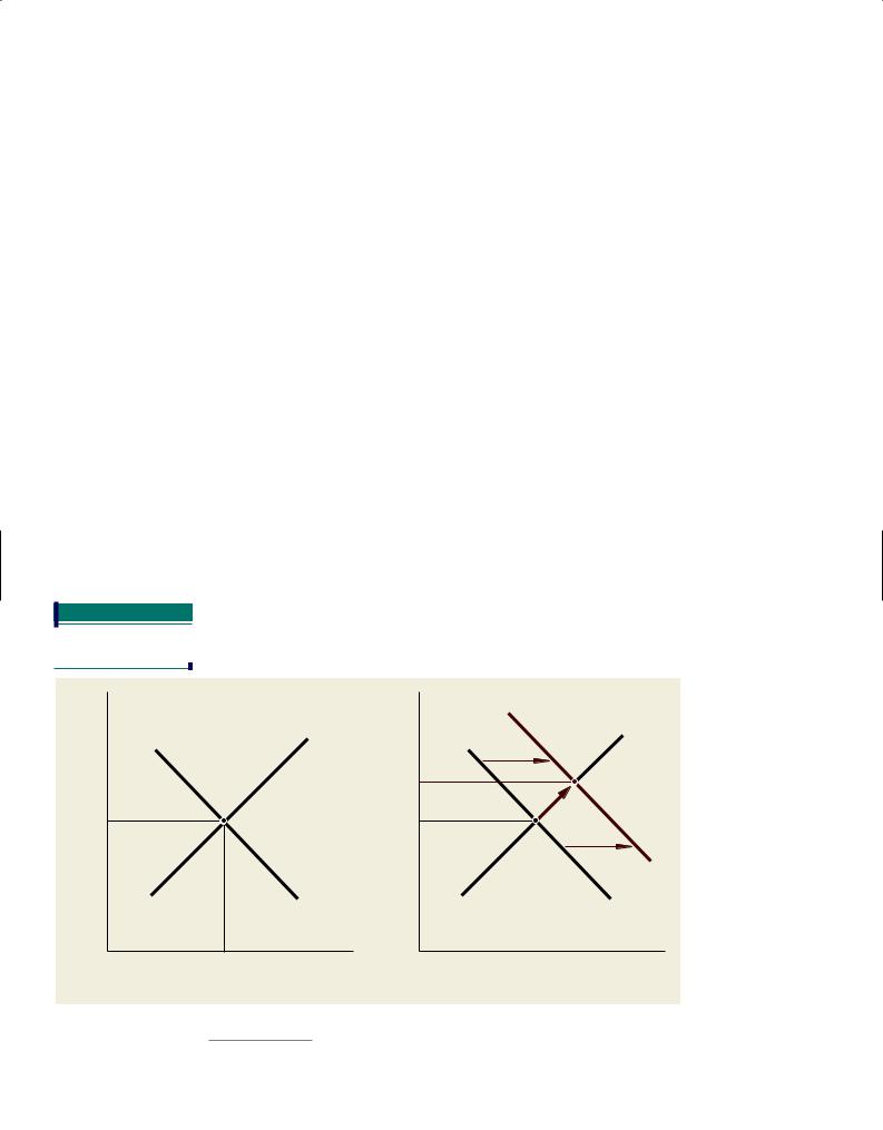
A Quick Review

Figure 1 shows two diagrams that should look familiar from Chapter 4. In Figure 1(a), we find a downward-sloping demand curve, labeled DD, and an upward-sloping supply curve, labeled SS. Because the figure is a multipurpose diagram, the “Price” and “Quantity” axes do not specify any particular commodity. To start on familiar terrain, first imagine that this graph depicts the market for milk, so the vertical axis measures the price of milk and the horizontal axis measures the quantity of milk demanded and supplied. As we know, if nothing interferes with the operation of a free market, equilibrium will be at point E with a price P0 and a quantity of output Q0.

Next, suppose something happens to shift the demand curve outward. For example, we learned in Chapter 4 that an increase in consumer incomes might do that. Figure 1(b) shows this shift as a rightward movement of the demand curve from D0D0 to D1D1. Equilibrium shifts from point E to point A, so both price and output rise.

Moving to Macroeconomic Aggregates

The aggregate demand curve shows the quantity of domestic product that is demanded at each possible value of the price level.

The aggregate supply curve shows the quantity of domestic product that is supplied at each possible value of the price level.

FIGURE 1

Two Interpretations of

a Shift in the Demand

Curve

Now let’s switch from microeconomics to macroeconomics. To do so, we reinterpret Figure 1 as representing the market for an abstract object called “domestic product”—one of those economic aggregates that we described earlier. No one has ever seen, touched, or eaten a unit of domestic product, but these are the kinds of abstractions we use in macroeconomic analysis.

Consistent with this reinterpretation, think of the price measured on the vertical axis as being another abstraction—the overall price index, or “cost of living.”1 Then the curve DD in Figure 1(a) is called an aggregate demand curve, and the curve SS is called an aggregate supply curve. We will develop an economic theory to derive these curves explicitly in Chapters 7 through 10. As we will see there, the curves have rather different origins from the microeconomic counterparts we encountered in Chapter 4.

					D1
			S		S
	D			D0
					A
				P1
Price		E	Price		E
	P0			P0
					D1
	S	D		S	D0
		Q0
		Quantity			Quantity
		(a)			(b)

1 The appendix to Chapter 6 explains how such price indexes are calculated.

Copyright 2009 Cengage Learning, Inc. All Rights Reserved. May not be copied, scanned, or duplicated, in whole or in part.