

Baumol & Blinder MACROECONOMICS (11th ed)
.pdfLICENSED TO:
CHAPTER 1 |
What Is Economics? |
7 |
up more than 1,000-fold in 200 years. It is estimated that rising labor productivity has increased the standard of living of a typical American worker approximately sevenfold in the past century (see Chapter 7).
Other economic issues such as unemployment, monopoly, and inequality are important to us all and will receive much attention in this book. But in the long run, nothing has as great an effect on our material well-being and the amounts society can afford to spend on hospitals, schools, and social amenities as the rate of growth of productivity—the amount that an average worker can produce in an hour. Chapter 7 points out that what appears to be a small increase in productivity growth can have a huge effect on a country’s standard of living over a long period of time because productivity compounds like the interest on savings in a bank. Similarly, a slowdown in productivity growth that persists for a substantial number of years can have a devastating effect on living standards.
Epilogue
These ideas are some of the more fundamental concepts you will find in this book—ideas that we hope you will retain beyond the final exam. There is no need to master them right now, for you will hear much more about each as you progress through the book. By the end of the course, you may be amazed to see how natural, or even obvious, they will seem.
INSIDE THE ECONOMIST’S TOOL KIT
We turn now from the kinds of issues economists deal with to some of the tools they use to grapple with them.
Economics as a Discipline
Although economics is clearly the most rigorous of the social sciences, it nevertheless looks decidedly more “social” than “scientific” when compared with, say, physics. An economist must be a jack of several trades, borrowing modes of analysis from numerous fields. Mathematical reasoning is often used in economics, but so is historical study. And neither looks quite the same as when practiced by a mathematician or a historian. Statistics play a major role in modern economic inquiry, although economists had to modify standard statistical procedures to fit their kinds of data.
The Need for Abstraction
Some students find economics unduly abstract and “unrealistic.” The stylized world envisioned by economic theory seems only a distant cousin to the world they know. There is an old joke about three people—a chemist, a physicist, and an economist— stranded on an desert island with an ample supply of canned food but no tools to open the cans. The chemist thinks that lighting a fire under the cans would burst the cans. The physicist advocates building a catapult with which to smash the cans against some boulders. The economist’s suggestion? “Assume a can opener.”
Economic theory does make some unrealistic assumptions; you will encounter some of them in this book. But some abstraction from reality is necessary because of the incredible complexity of the economic world, not because economists like to sound absurd.
Compare the chemist’s simple task of explaining the interactions of compounds in a chemical reaction with the economist’s
SOURCE: From The Wall Street Journal. Permission, Cartoon Features Syndicate.
”Yes, John, we’d all like to make economics less dismal . . . “
NOTE: The nineteenth-century British writer Thomas Carlyle described economics as the “dismal science,” a label that stuck.
Copyright 2009 Cengage Learning, Inc. All Rights Reserved. May not be copied, scanned, or duplicated, in whole or in part.

LICENSED TO:
8 |
PART 1 |
Getting Acquainted with Economics |
ABSTRACTION means ignoring many details so as to focus on the most important elements of a problem.
complex task of explaining the interactions of people in an economy. Are molecules motivated by greed or altruism, by envy or ambition? Do they ever imitate other molecules? Do forecasts about them influence their behavior? People, of course, do all these things and many, many more. It is therefore vastly more difficult to predict human behavior than to predict chemical reactions. If economists tried to keep track of every feature of human behavior, they would never get anywhere. Thus:
Abstraction from unimportant details is necessary to understand the functioning of anything as complex as the economy.
An analogy will make clear why economists abstract from details. Suppose you have just arrived for the first time in Los Angeles. You are now at the Los Angeles Civic Center—the point marked A in Maps 1 and 2, which are alternative maps of part of Los Angeles. You want to drive to the Los Angeles County Museum of Art, point B on each map. Which map would be more useful?
Map 1 has complete details of the Los Angeles road system. This makes it hard to read and hard to use as a way to find the art museum. For this purpose, Map 1 is far too detailed, although for some other purposes (for example, locating some small street in Hollywood) it may be far better than Map 2.
In contrast, Map 2 omits many minor roads—you might say they are assumed away—so that the freeways and major arteries stand out more clearly. As a result of this simplification, several routes from the Civic Center to the Los Angeles County Museum of Art emerge. For example, we can take the Hollywood Freeway west to Alvarado Boulevard, go south to Wilshire Boulevard, and then head west again. Although we might find a shorter route by poring over the details in Map 1, most strangers to the city would be better off with Map 2. Similarly, economists try to abstract from a lot of confusing details while retaining the essentials.
Map 3, however, illustrates that simplification can go too far. It shows little more than the major interstate routes that pass through the greater Los Angeles area and therefore
MAP 1
Detailed Road Map of Los Angeles
Map © by Rand McNally, RL. 08-S-32. Reprinted by permission.
NOTE: Point A marks the Los Angeles Civic Center and Point B marks the Los Angeles County Museum of Art.
Copyright 2009 Cengage Learning, Inc. All Rights Reserved. May not be copied, scanned, or duplicated, in whole or in part.

LICENSED TO:
CHAPTER 1 |
What Is Economics? |
9 |
will not help a visitor find the art museum. Of course, this map was never intended to be used as a detailed tourist guide, which brings us to an important point:
There is no such thing as one “right” degree of abstraction and simplification for all analytic purposes. The proper degree of abstraction depends on the objective of the analysis. A model that is a gross oversimplification for one purpose may be needlessly complicated for another.
Economists are constantly seeking analogies to Map 2 rather than Map 3, treading the thin line between useful generalizations about complex issues and gross distortions of the pertinent facts. For example, suppose you want to learn why some people are fabulously rich while others are abjectly poor. People differ in many ways, too many to enumerate, much less to study. The economist must ignore most of these details to focus on the important ones. The color of a person’s hair or eyes is probably not important for the problem but, unfortunately, the color of his or her skin probably is because racial discrimination can depress a person’s income. Height and weight may not matter, but education probably does. Proceeding in this way, we can pare Map 1 down to the manageable dimensions of Map 2. But there is a danger of going too far, stripping away some of the crucial factors, so that we wind up with Map 3.
 MAP 2
MAP 2
Major Los Angeles Arteries and Freeways
Map © by Rand McNally, R.L.04-S-14. Reprinted by permission.
 MAP 3
MAP 3
Greater Los Angeles Freeways
Transportation
The Role of |
of |
|
Department |
||
Economic Theory |
||
|
||
Some students find economics |
California |
|
“too theoretical.” To see why we |
||
|
||
can’t avoid it, let’s consider what |
SOURCE: |
|
we mean by a theory. |
||
|
||
To an economist or natural sci- |
|
|
entist, the word theory means |
|
something different from what it means in common speech. In science, a theory is not an untested assertion of alleged fact. The statement that aspirin provides protection against heart attacks is not a theory; it is a hypothesis, that is, a reasoned guess, which will prove
A theory is a deliberate simplification of relationships used to explain how those relationships work.
Copyright 2009 Cengage Learning, Inc. All Rights Reserved. May not be copied, scanned, or duplicated, in whole or in part.

LICENSED TO:
10 |
PART 1 |
Getting Acquainted with Economics |
Two variables are said to be correlated if they tend to go up or down together.
Correlation need not imply causation.
An economic model is a simplified, small-scale version of some aspect of the economy. Economic models are often expressed in equations, by graphs, or
in words.
to be true or false once the right sorts of experiments have been completed. But a theory is different. It is a deliberate simplification (abstraction) of reality that attempts to explain how some relationships work. It is an explanation of the mechanism behind observed phenomena. Thus, gravity forms the basis of theories that describe and explain the paths of the planets. Similarly, Keynesian theory (discussed in Parts 2 and 3) seeks to describe and explain how government policies affect unemployment and prices in the national economy.
People who have never studied economics often draw a false distinction between theory and practical policy. Politicians and businesspeople, in particular, often reject abstract economic theory as something that is best ignored by “practical” people. The irony of these statements is that
It is precisely the concern for policy that makes economic theory so necessary and important.
To analyze policy options, economists are forced to deal with possibilities that have not actually occurred. For example, to learn how to shorten periods of high unemployment, they must investigate whether a proposed new policy that has never been tried can help. Or to determine which environmental programs will be most effective, they must understand how and why a market economy produces pollution and what might happen if the government taxed industrial waste discharges and automobile emissions. Such questions require some theorizing, not just examination of the facts, because we need to consider possibilities that have never occurred.
The facts, moreover, can sometimes be highly misleading. Data often indicate that two variables move up and down together. But this statistical correlation does not prove that either variable causes the other. For example, when it rains, people drive their cars more slowly and there are also more traffic accidents. But no one thinks that it is the slower driving that causes more accidents when it’s raining. Rather, we understand that both phenomena are caused by a common underlying factor—more rain. How do we know this? Not just by looking at the correlation between data on accidents and driving speeds. Data alone tell us little about cause and effect. We must use some simple theory as part of our analysis. In this case, the theory might explain that drivers are more apt to have accidents on rain-slicked roads.
Similarly, we must use theoretical analysis, and not just data alone, to understand how, if at all, different government policies will lead to lower unemployment or how a tax on emissions will reduce pollution.
Statistical correlation need not imply causation. Some theory is usually needed to interpret data.
What Is an Economic Model?
An economic model is a representation of a theory or a part of a theory, often used to gain insight into cause and effect. The notion of a “model” is familiar enough to children; and economists—like other researchers—use the term in much the same way that children do.
A child’s model airplane looks and operates much like the real thing, but it is much smaller and simpler, so it is easier to manipulate and understand. Engineers for Boeing also build models of planes. Although their models are far larger and much more elaborate than a child’s toy, they use them for much the same purposes: to observe the workings of these aircraft “up close” and to experiment with them to see how the models behave under different circumstances. (“What happens if I do this?”) From these experiments, they make educated guesses as to how the real-life version will perform.
Economists use models for similar purposes. The late A. W. Phillips, the famous engineer-turned-economist who discovered the “Phillips curve” (discussed in Chapter 16), was talented enough to construct a working model of the determination of national
Copyright 2009 Cengage Learning, Inc. All Rights Reserved. May not be copied, scanned, or duplicated, in whole or in part.

LICENSED TO:
CHAPTER 1 |
What Is Economics? |
11 |
income in a simple economy by using colored water flowing through pipes. For years this contraption has graced the basement of the London School of Economics. Although we will explain the models with words and diagrams, Phillips’s engineering background enabled him to depict the theory with tubes, valves, and pumps.
Because many of the models used in this book are depicted in diagrams, for those of you who need review, we explain the construction and use of various types of graphs in the appendix to this chapter. Don’t be put off by seemingly abstract models. Think of them as useful road maps. And remember how hard it would be to find your way around Los Angeles without one.
Reasons for Disagreements: Imperfect
Information and Value Judgments
“If all the earth’s economists were laid end to end, they could not reach an agreement,” the saying goes. Politicians and reporters are fond of pointing out that economists can be found on both sides of many public policy issues. If economics is a science, why do economists so often disagree? After all, astronomers do not debate whether the earth revolves around the sun or vice versa.
This question reflects a misunderstanding of the nature of sci-
ence. Disputes are normal at the frontier of any science. For example, astronomers once did argue vociferously over whether the earth revolves around the sun. Nowadays, they argue about gamma-ray bursts, dark matter, and other esoterica. These arguments go mostly unnoticed by the public because few of us understand what they are talking about. But economics is a social science, so its disputes are aired in public and all sorts of people feel competent to join economic debates.
Furthermore, economists actually agree on much more than is commonly supposed. Virtually all economists, regardless of their politics, agree that taxing polluters is one of the best ways to protect the environment, that rent controls can ruin a city (Chapter 4), and that free trade among nations is usually preferable to the erection of barriers through tariffs and quotas (see Chapter 17). The list could go on and on. It is probably true that the issues about which economists agree far exceed the subjects on which they disagree.
Finally, many disputes among economists are not scientific disputes at all. Sometimes the pertinent facts are simply unknown. For example, you will learn in Chapter 17 that the appropriate financial penalty to levy on a polluter depends on quantitative estimates of the harm done by the pollutant. But good estimates of this damage may not be available. Similarly, although there is wide scientific agreement that the earth is slowly warming, there are disagreements over how costly global warming may be. Such disputes make it difficult to agree on a concrete policy proposal.
Another important source of disagreements is that economists, like other people, come in all political stripes: conservative, middle-of-the-road, liberal, radical. Each may have different values, and so each may hold a different view of the “right” solution to a public policy problem—even if they agree on the underlying analysis. Here are two examples:
1.We suggested early in this chapter that policies that lower inflation are likely to raise unemployment. Many economists believe they can measure the amount of unemployment that must be endured to reduce inflation by a given amount. But they disagree about whether it is worth having, say, three million more people out of work for a year to cut the inflation rate by 1 percent.
Copyright 2009 Cengage Learning, Inc. All Rights Reserved. May not be copied, scanned, or duplicated, in whole or in part.

LICENSED TO:
12PART 1 Getting Acquainted with Economics
2.In designing an income tax, society must decide how much of the burden to put on upper-income taxpayers. Some people believe the rich should pay a disproportionate share of the taxes. Others disagree, believing it is fairer to levy the same income tax rate on everyone.
Economists cannot answer questions like these any more than nuclear physicists could have determined whether dropping the atomic bomb on Hiroshima was a good idea. The decisions rest on moral judgments that can be made only by the citizenry through its elected officials.
Although economic science can contribute theoretical and factual knowledge on a particular issue, the final decision on policy questions often rests either on information that is not currently available or on social values and ethical opinions about which people differ, or on both.
| SUMMARY |
1.To help you get the most out of your first course in economics, we have devised a list of seven important ideas that you will want to retain beyond the final exam. Briefly, they are the following:
a.Opportunity cost is the correct measure of cost.
b.Attempts to fight market forces often backfire.
c.Nations can gain from trade by exploiting their comparative advantages.
d.Both parties can gain in a voluntary exchange.
e.Governments have tools that can mitigate cycles of boom and bust, but these tools are imperfect.
f.In the short run, policy makers face a trade-off between inflation and unemployment. Policies that reduce one normally increase the other.
g.In the long run, productivity is almost the only thing that matters for a society’s material well-being.
2.Common sense is not always a reliable guide in explaining economic issues or in making economic decisions.
3.Because of the great complexity of human behavior, economists are forced to abstract from many details, to make generalizations that they know are not quite true, and to organize what knowledge they have in terms of some theoretical structure called a “model.”
4.Correlation need not imply causation.
5.Economists use simplified models to understand the real world and predict its behavior, much as a child uses a model railroad to learn how trains work.
6.Although these models, if skillfully constructed, can illuminate important economic problems, they rarely can answer the questions that confront policy makers. Value judgments involving such matters as ethics are needed for this purpose, and the economist is no better equipped than anyone else to make them.
| KEY TERMS |
Opportunity cost 4 |
Theory 9 |
Economic model 10 |
Abstraction 8 |
Correlation |
10 |
| DISCUSSION QUESTIONS |
1.Think about how you would construct a model of how your college is governed. Which officers and administrators would you include and exclude from your model if the objective were one of the following:
a.To explain how decisions on financial aid are made
b.To explain the quality of the faculty
Relate this to the map example in the chapter.
2.Relate the process of abstraction to the way you take notes in a lecture. Why do you not try to transcribe every word uttered by the lecturer? Why don’t you write down just the title of the lecture and stop there? How do you decide, roughly speaking, on the correct amount of detail?
3.Explain why a government policy maker cannot afford to ignore economic theory.
Copyright 2009 Cengage Learning, Inc. All Rights Reserved. May not be copied, scanned, or duplicated, in whole or in part.
LICENSED TO:
CHAPTER 1 |
What Is Economics? |
13 |
| APPENDIX | Using Graphs: A Review1
As noted in the chapter, economists often explain and analyze models with the help of graphs. Indeed, this book is full of them. But that is not the only reason for studying how graphs work. Most college students will deal with graphs in the future, perhaps frequently. You will see them in newspapers. If you become a doctor, you will use graphs to keep track of your patients’ progress. If you join a business firm, you will use them to check profit or performance at a glance. This appendix introduces some of the techniques of graphic analysis—tools you will use throughout the book and, more important, very likely throughout your working career.
GRAPHS USED IN ECONOMIC ANALYSIS
Economic graphs are invaluable because they can display a large quantity of data quickly and because they facilitate data interpretation and analysis. They enable the eye to take in at a glance important statistical relationships that would be far less apparent from written descriptions or long lists of numbers.
TWO-VARIABLE DIAGRAMS
Much of the economic analysis found in this and other books requires that we keep track of two variables simultaneously.
FIGURE 1
A variable is something measured by a number; it is used to analyze what happens to other things when the size of that number changes (varies).
For example, in studying how markets operate, we will want to keep one eye on the price of a commodity and the other on the quantity of that commodity that is bought and sold.
For this reason, economists frequently find it useful to display real or imaginary figures in a two-variable diagram, which simultaneously represents the behavior of two economic variables. The numerical value of one variable is measured along the horizontal line at the bottom of the graph (called the horizontal axis), starting from the origin (the point labeled “0”), and the numerical value of the other variable is measured up the vertical line on the left side of the graph (called the vertical axis), also starting from the origin.
The “0” point in the lower-left corner of a graph where the axes meet is called the origin. Both variables are equal to zero at the origin.
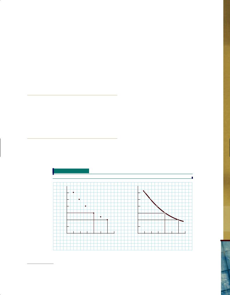
Figures 1(a) and 1(b) are typical graphs of economic analysis. They depict an imaginary demand curve, represented by the brick-colored dots in Figure 1(a) and the heavy brick-colored line in Figure 1(b). The graphs show the price of natural gas on their vertical axes and the quantity of gas people want to buy at each price on the horizontal axes. The dots in Figure 1(a) are
A Hypothetical Demand Curve for Natural Gas in St. Louis
Price
|
|
|
|
|
|
|
|
D |
|
|
|
|
6 |
|
|
|
|
|
|
6 |
|
|
|
|
|
5 |
|
|
|
|
|
|
5 |
|
|
|
|
|
4 |
|
|
|
|
|
Price |
4 |
|
|
|
|
|
3 |
P |
|
|
A |
|
3 |
P |
|
|
A |
|
|
|
|
|
|
|
|
|
||||||
|
|
|
|
|
|
|
|
|
|
|
||
|
|
|
|
|
B |
|
|
|
|
|
|
B |
2 |
|
|
|
|
|
|
2 |
|
|
|
|
D |
|
|
|
|
|
|
|
|
|
|
|
|
|
1 |
|
|
|
|
|
|
1 |
|
|
|
|
|
|
|
|
|
Q |
|
|
|
|
|
|
Q |
|
0 |
20 |
40 |
60 |
80 |
100 120 140 |
|
0 |
20 |
40 |
60 |
80 |
100 120 140 |
|
|
|
Quantity |
|
|
|
|
|
Quantity |
|
||
|
|
|
(a) |
|
|
|
|
|
(b) |
|
||
NOTE: Price is in dollars per thousand cubic feet; quantity is in billions of cubic feet per year.
1 Students who have some acquaintance with geometry and feel quite comfortable with graphs can safely skip this appendix.
Copyright 2009 Cengage Learning, Inc. All Rights Reserved. May not be copied, scanned, or duplicated, in whole or in part.

LICENSED TO:
14 PART 1 Getting Acquainted with Economics
connected by the continuous brick-colored curve labeled DD in Figure 1(b).
Economic diagrams are generally read just as one would read latitudes and longitudes on a map. On the demand curve in Figure 1, the point marked a represents a hypothetical combination of price and quantity of natural gas demanded by customers in St. Louis. By drawing a horizontal line leftward from that point to the vertical axis, we learn that at this point the average price for gas in St. Louis is $3 per thousand cubic feet. By dropping a line straight down to the horizontal axis, we find that consumers want 80 billion cubic feet per year at this price, just as the statistics in Table 1 show. The other points on the graph give similar information. For example, point b indicates that if natural gas in St. Louis were to cost only $2 per thousand cubic feet, quantity demanded would be higher—it would reach 120 billion cubic feet per year.
TABLE 1
Quantities of Natural Gas Demanded at Various Prices
|
Price (per thousand |
|
|
|
|
|
|
|
cubic feet) |
$2 |
$3 |
$4 |
$5 |
$6 |
|
|
Quantity demanded (billions |
|
|
|
|
|
|
|
of cubic feet per year) |
120 |
80 |
56 |
38 |
20 |
|
|
|
|
|
|
|
|
|
|
|
|
|
|
|
|
|
Notice that information about price and quantity is all we can learn from the diagram. The demand curve will not tell us what kinds of people live in St. Louis, the sizes of their homes, or the condition of their furnaces. It tells us about the quantity demanded at each possible price—no more, no less.
A diagram abstracts from many details, some of which may be quite interesting, so as to focus on the two variables of primary interest—in this case, the price of natural gas and the amount of gas that is demanded at each price. All of the diagrams used in this book share this basic feature. They cannot tell the reader the
“whole story,” any more than a map’s latitude and longitude figures for a particular city can make someone an authority on that city.
THE DEFINITION AND MEASUREMENT OF SLOPE
One of the most important features of economic diagrams is the rate at which the line or curve being sketched runs uphill or downhill as we move to the right. The demand curve in Figure 1 clearly slopes downhill (the price falls) as we follow it to the right (that is, as consumers demand more gas). In such instances, we say that the curve has a negative slope, or is negatively sloped, because one variable falls as the other one rises.
The slope of a straight line is the ratio of the vertical change to the corresponding horizontal change as we move to the right along the line between two points on that line, or, as it is often said, the ratio of the “rise” over the “run.”
The four panels of Figure 2 show all possible types of slope for a straight-line relationship between two unnamed variables called Y (measured along the vertical axis) and X (measured along the horizontal axis). Figure 2(a) shows a negative slope, much like our demand curve in the previous graph. Figure 2(b) shows a positive slope, because variable Y rises (we go uphill) as variable X rises (as we move to the right). Figure 2(c) shows a zero slope, where the value of Y is the same irrespective of the value of X. Figure 2(d) shows an infinite slope, meaning that the value of X is the same irrespective of the value of Y.
Slope is a numerical concept, not just a qualitative one. The two panels of Figure 3 show two positively sloped straight lines with different slopes. The line in Figure 3(b) is clearly steeper. But by how much? The labels should help you compute the answer. In
FIGURE 2
Different Types of Slope of a Straight-Line Graph
Y Y Y Y
|
|
|
|
|
|
|
|
|
|
|
|
|
Negative |
|
Positive |
|
Zero |
|
|
|
|
Infinite |
|
|
slope |
|
slope |
|
slope |
|
|
|
|
slope |
|
|
|
X |
|
X |
|
|
X |
|
|
|
X |
|
|
|
|
|
|
|
|||||
0 |
|
0 |
|
0 |
|
|
|
0 |
|
|
|
|
(a) |
|
(b) |
|
(c) |
|
|
|
(d) |
||
Copyright 2009 Cengage Learning, Inc. All Rights Reserved. May not be copied, scanned, or duplicated, in whole or in part.

LICENSED TO:
CHAPTER 1 |
What Is Economics? |
15 |
FIGURE 3
How to Measure Slope
|
Y |
|
|
|
Y |
|
|
|
|
|
|
|
3 |
|
|
|
|
|
|
Slope = — |
|
|
|
|
|
|
10 |
|
|
|
|
|
|
C |
|
|
|
|
11 |
|
|
9 |
|
C |
1 |
|
|
|
|
|
|
|
|
||
8 |
|
|
Slope = — |
8 |
|
B |
A |
B |
10 |
A |
|||
|
|
|
|
|||
|
|
|
|
|
||
|
|
|
X |
|
|
X |
0 |
3 |
13 |
|
0 |
3 |
13 |
|
|
(a) |
|
|
|
(b) |
Figure 3(a) a horizontal movement, AB, of 10 units (13 2 3) corresponds to a vertical movement, BC, of 1 unit (9 2 8). So the slope is BC/AB 5 1/10. In Figure 3(b), the same horizontal movement of 10 units corresponds to a vertical movement of 3 units (11 2 8). So the slope is 3/10, which is larger—the rise divided by the run is greater in Figure 3(b).
By definition, the slope of any particular straight line remains the same, no matter where on that line we choose to measure it. That is why we can pick any horizontal distance, AB, and the corresponding slope triangle, ABC, to measure slope. But this is not true for curved lines.
Curved lines also have slopes, but the numerical value of the slope differs at every point along the curve as we move from left to right.
The four panels of Figure 4 provide some examples of slopes of curved lines. The curve in Figure 4(a)
has a negative slope everywhere, and the curve in Figure 4(b) has a positive slope everywhere. But these are not the only possibilities. In Figure 4(c) we encounter a curve that has a positive slope at first but a negative slope later on. Figure 4(d) shows the opposite case: a negative slope followed by a positive slope.
We can measure the slope of a smooth curved line numerically at any particular point by drawing a straight line that touches, but does not cut, the curve at the point in question. Such a line is called a tangent to the curve.
The slope of a curved line at a particular point is defined as the slope of the straight line that is tangent to the curve at that point.
Figure 5 shows tangents to the brick-colored curve at two points. Line tt is tangent at point T, and line rr is tangent at point R. We can measure the slope of the
 FIGURE 4
Behavior of Slopes in Curved Graphs
Y |
Y |
Y |
Y |
||||||||
|
|
|
|
|
|
|
Negative |
|
Positive |
||
|
|
|
|
|
|
|
slope |
|
slope |
||
|
Negative |
|
Positive |
|
|
|
|
|
|
||
|
slope |
|
slope |
|
|
|
|
Negative |
|||
|
|
|
|
|
|
|
Positive |
|
slope |
||
|
|
|
|
|
|
|
slope |
|
|
|
|
0 |
|
X |
0 |
|
X |
0 |
|
X |
0 |
|
X |
|
|
|
|
||||||||
|
|
|
|
|
|
|
|
||||
|
(a) |
|
(b) |
|
(c) |
|
(d) |
||||
|
|
|
|
|
|
|
|
|
|
|
|
Copyright 2009 Cengage Learning, Inc. All Rights Reserved. May not be copied, scanned, or duplicated, in whole or in part.

LICENSED TO:
16 |
PART 1 |
Getting Acquainted with Economics |
FIGURE 5
How to Measure Slope at a Point on a Curved Graph
|
Y |
|
|
|
|
|
|
|
|
|
8 |
|
|
|
|
R |
|
|
|
|
|
|
|
|
|
|
|
|
|
|
|
|
7 |
|
|
|
|
|
D |
|
|
|
|
|
|
|
|
|
|
|
|
|
|
|
6 |
T |
|
|
|
|
|
|
|
|
|
|
|
|
|
|
|
|
|
|
|
|
5 |
|
|
|
|
|
|
|
F |
|
|
C |
|
|
|
|
E |
|
|
|
|
|
|
|
|
|
|
|
|
|
|
||
4 |
|
|
|
|
|
|
|
|
R |
|
3 |
|
|
|
|
|
|
|
|
|
|
2 |
|
|
|
|
|
|
|
|
|
|
1 |
B |
|
|
A |
|
|
|
|
|
|
|
|
|
|
|
|
|
|
|
|
|
|
|
|
|
T |
|
|
|
|
|
X |
|
|
|
|
|
|
|
|
|
|
|
0 |
1 |
2 |
3 |
4 |
5 |
6 |
7 |
8 |
9 |
10 |
curve at these two points by applying the definition. The calculation for point T, then, is the following:
Slope at point T 5 Slope of line TT
Distance BC
5 Distance BA
11 2 52 |
24 |
5 22 |
||
5 |
13 2 12 |
5 |
2 |
|
A similar calculation yields the slope of the curve at point R, which, as we can see from Figure 5, must be smaller numerically. That is, the tangent line rr is less steep than line tt:
Slope at point R 5 Slope of line RR
15 2 72 |
22 |
5 21 |
||
5 |
18 2 62 |
5 |
2 |
|
Exercise Show that the slope of the curve at point G is about 1.
What would happen if we tried to apply this graphical technique to the high point in Figure 4(c) or to the low point in Figure 4(d)? Take a ruler and try it. The tangents that you construct should be horizontal, meaning that they should have a slope exactly equal to zero. It is always true that where the slope of a smooth curve changes from positive to negative, or vice versa, there will be at least one point whose slope is zero.
Curves shaped like smooth hills, as in Figure 4(c), have a zero slope at their highest point. Curves shaped like valleys, as in Figure 4(d), have a zero slope at their lowest point.
RAYS THROUGH THE ORIGIN
AND 45° LINES
The point at which a straight line cuts the vertical (Y) axis is called the Y-intercept.
The Y-intercept of a line or a curve is the point at which it touches the vertical axis (the Y-axis). The X-intercept is defined similarly.
For example, the Y-intercept of the line in Figure 3(a) is a bit less than 8.
Lines whose Y-intercept is zero have so many special uses in economics and other disciplines that they have been given a special name: a ray through the origin, or a ray.
Figure 6 shows three rays through the origin, and the slope of each is indicated in the diagram. The ray in the center (whose slope is 1) is particularly useful in many economic applications because it marks points where X and Y are equal (as long as X and Y are measured in the same units). For example, at point A we have X 5 3 and Y 5 3; at point B, X 5 4 and Y 5 4. A similar relation holds at any other point on that ray.
How do we know that this is always true for a ray whose slope is 1? If we start from the origin (where both X and Y are zero) and the slope of the ray is 1, we know from the definition of slope that
Vertical change
Slope 5 Horizontal change 5 1
This implies that the vertical change and the horizontal change are always equal, so the two variables
 FIGURE 6
Rays Through the Origin
|
Y |
|
|
|
|
|
|
5 |
|
|
|
Slope = + 2 |
|
|
|
|
|
|
|
|
|
|
|
4 |
|
|
|
|
|
Slope = + 1 |
|
|
|
|
|
B |
|
|
|
|
|
|
|
|
|
|
|
3 |
C |
|
|
A |
|
|
|
|
|
|
|
|
|
|
|
2 |
|
|
K |
|
Slope = + |
1 |
|
|
|
|
|
– |
|||
|
|
|
|
|
|
|
2 |
1 |
|
|
E |
|
|
|
|
|
|
|
|
|
|
|
|
|
|
|
|
D |
|
|
X |
|
0 |
1 |
2 |
3 |
4 |
5 |
|
|
|
||||||
Copyright 2009 Cengage Learning, Inc. All Rights Reserved. May not be copied, scanned, or duplicated, in whole or in part.