Mankiw Principles of Macroeconomics (3rd ed)

32 PART ONE INTRODUCTION

DIFFERENCES IN VALUES

Suppose that Peter and Paul both take the same amount of water from the town well. To pay for maintaining the well, the town taxes its residents. Peter has income of $50,000 and is taxed $5,000, or 10 percent of his income. Paul has income of $10,000 and is taxed $2,000, or 20 percent of his income.

Is this policy fair? If not, who pays too much and who pays too little? Does it matter whether Paul’s low income is due to a medical disability or to his decision to pursue a career in acting? Does it matter whether Peter’s high income is due to a large inheritance or to his willingness to work long hours at a dreary job?

These are difficult questions on which people are likely to disagree. If the town hired two experts to study how the town should tax its residents to pay for the well, we would not be surprised if they offered conflicting advice.

This simple example shows why economists sometimes disagree about public policy. As we learned earlier in our discussion of normative and positive analysis, policies cannot be judged on scientific grounds alone. Economists give conflicting advice sometimes because they have different values. Perfecting the science of economics will not tell us whether it is Peter or Paul who pays too much.

PERCEPTION VERSUS REALITY

Because of differences in scientific judgments and differences in values, some disagreement among economists is inevitable. Yet one should not overstate the amount of disagreement. In many cases, economists do offer a united view.

Table 2-2 contains ten propositions about economic policy. In a survey of economists in business, government, and academia, these propositions were endorsed by an overwhelming majority of respondents. Most of these propositions would fail to command a similar consensus among the general public.

The first proposition in the table is about rent control. For reasons we will discuss in Chapter 6, almost all economists believe that rent control adversely affects the availability and quality of housing and is a very costly way of helping the most needy members of society. Nonetheless, many city governments choose to ignore the advice of economists and place ceilings on the rents that landlords may charge their tenants.

The second proposition in the table concerns tariffs and import quotas. For reasons we will discuss in Chapter 3 and more fully in Chapter 9, almost all economists oppose such barriers to free trade. Nonetheless, over the years, the president and Congress have chosen to restrict the import of certain goods. In 1993 the North American Free Trade Agreement (NAFTA), which reduced barriers to trade among the United States, Canada, and Mexico, passed Congress, but only by a narrow margin, despite overwhelming support from economists. In this case, economists did offer united advice, but many members of Congress chose to ignore it.

Why do policies such as rent control and import quotas persist if the experts are united in their opposition? The reason may be that economists have not yet convinced the general public that these policies are undesirable. One purpose of this book is to make you understand the economist’s view of these and other subjects and, perhaps, to persuade you that it is the right one.

CHAPTER 2 THINKING LIKE AN ECONOMIST

33

PROPOSITION (AND PERCENTAGE OF ECONOMISTS WHO AGREE)

1.A ceiling on rents reduces the quantity and quality of housing available. (93%)

2.Tariffs and import quotas usually reduce general economic welfare. (93%)

3.Flexible and floating exchange rates offer an effective international monetary arrangement. (90%)

4.Fiscal policy (e.g., tax cut and/or government expenditure increase) has a significant stimulative impact on a less than fully employed economy. (90%)

5.If the federal budget is to be balanced, it should be done over the business cycle rather than yearly. (85%)

6.Cash payments increase the welfare of recipients to a greater degree than do transfers-in-kind of equal cash value. (84%)

7.A large federal budget deficit has an adverse effect on the economy. (83%)

8.A minimum wage increases unemployment among young and unskilled workers. (79%)

9.The government should restructure the welfare system along the lines of a “negative income tax.” (79%)

10.Effluent taxes and marketable pollution permits represent a better approach to pollution control than imposition of pollution ceilings. (78%)

SOURCE: Richard M. Alston, J. R. Kearl, and Michael B. Vaughn, “Is There Consensus among Economists in the 1990s?” American Economic Review (May 1992): 203–209.

QUICK QUIZ: Why might economic advisers to the president disagree about a question of policy?

LET’S GET GOING

The first two chapters of this book have introduced you to the ideas and methods of economics. We are now ready to get to work. In the next chapter we start learning in more detail the principles of economic behavior and economic policy.

As you proceed through this book, you will be asked to draw on many of your intellectual skills. You might find it helpful to keep in mind some advice from the great economist John Maynard Keynes:

The study of economics does not seem to require any specialized gifts of an unusually high order. Is it not . . . a very easy subject compared with the higher branches of philosophy or pure science? An easy subject, at which very few excel! The paradox finds its explanation, perhaps, in that the master-economist must possess a rare combination of gifts. He must be mathematician, historian, statesman, philosopher—in some degree. He must understand symbols and speak in words. He must contemplate the particular in terms of the general, and touch abstract and concrete in the same flight of thought. He must study the

Table 2-2

TEN PROPOSITIONS ABOUT

WHICH MOST ECONOMISTS

AGREE

34 PART ONE INTRODUCTION

present in the light of the past for the purposes of the future. No part of man’s nature or his institutions must lie entirely outside his regard. He must be purposeful and disinterested in a simultaneous mood; as aloof and incorruptible as an artist, yet sometimes as near the earth as a politician.

It is a tall order. But with practice, you will become more and more accustomed to thinking like an economist.

Summar y

Economists try to address their objectivity. Like all scientists, they assumptions and build simplified understand the world around economic models are the circular production possibilities frontier.

The field of economics is divided microeconomics and macroeconomics study decisionmaking by households interaction among households marketplace. Macroeconomists trends that affect the economy

is an assertion about how the statement is an assertion about to be. When economists make

they are acting more as policy

.

advise policymakers offer conflicting of differences in scientific

of differences in values. At other are united in the advice they offer, but choose to ignore it.

		Key Concepts
circular-flow diagram, p. 23		positive statements, p. 29
production possibilities frontier, p. 25		normative statements, p. 29

Questions for Review

1.How is economics like a science?

2.Why do economists make assumptions?

3.Should an economic model describe reality exactly?

4.Draw and explain a production possibilities frontier for an economy that produces milk and cookies. What happens to this frontier if disease kills half of the economy’s cow population?

5.Use a production possibilities frontier to describe the idea of “efficiency.”

6.What are the two subfields into which economics is divided? Explain what each subfield studies.

7.What is the difference between a positive and a normative statement? Give an example of each.

8.What is the Council of Economic Advisers?

9.Why do economists sometimes offer conflicting advice to policymakers?

CHAPTER 2 THINKING LIKE AN ECONOMIST

35

Problems and Applications

1.Describe some unusual language used in one of the other fields that you are studying. Why are these special terms useful?

2.One common assumption in economics is that the products of different firms in the same industry are indistinguishable. For each of the following industries, discuss whether this is a reasonable assumption.

a.steel

b.novels

c.wheat

d.fast food

3.Draw a circular-flow diagram. Identify the parts of the model that correspond to the flow of goods and services and the flow of dollars for each of the following activities.

a.Sam pays a storekeeper $1 for a quart of milk.

b.Sally earns $4.50 per hour working at a fast food restaurant.

c.Serena spends $7 to see a movie.

d.Stuart earns $10,000 from his 10 percent ownership of Acme Industrial.

4.Imagine a society that produces military goods and consumer goods, which we’ll call “guns” and “butter.”

a.Draw a production possibilities frontier for guns and butter. Explain why it most likely has a bowedout shape.

b.Show a point that is impossible for the economy to achieve. Show a point that is feasible but inefficient.

c.Imagine that the society has two political parties, called the Hawks (who want a strong military) and the Doves (who want a smaller military). Show a point on your production possibilities frontier that the Hawks might choose and a point the Doves might choose.

d.Imagine that an aggressive neighboring country reduces the size of its military. As a result, both the Hawks and the Doves reduce their desired production of guns by the same amount. Which party would get the bigger “peace dividend,” measured by the increase in butter production? Explain.

5.The first principle of economics discussed in Chapter 1 is that people face tradeoffs. Use a production possibilities frontier to illustrate society’s tradeoff between a clean environment and high incomes. What do you suppose determines the shape and position of the frontier? Show what happens to the frontier if

engineers develop an automobile engine with almost no emissions.

6.Classify the following topics as relating to microeconomics or macroeconomics.

a.a family’s decision about how much income to save

b.the effect of government regulations on auto emissions

c.the impact of higher national saving on economic growth

d.a firm’s decision about how many workers to hire

e.the relationship between the inflation rate and changes in the quantity of money

7.Classify each of the following statements as positive or normative. Explain.

a.Society faces a short-run tradeoff between inflation and unemployment.

b.A reduction in the rate of growth of money will reduce the rate of inflation.

c.The Federal Reserve should reduce the rate of growth of money.

d.Society ought to require welfare recipients to look for jobs.

e.Lower tax rates encourage more work and more saving.

8.Classify each of the statements in Table 2-2 as positive, normative, or ambiguous. Explain.

9.If you were president, would you be more interested in your economic advisers’ positive views or their normative views? Why?

10.The Economic Report of the President contains statistical information about the economy as well as the Council of Economic Advisers’ analysis of current policy issues. Find a recent copy of this annual report at your library and read a chapter about an issue that interests you. Summarize the economic problem at hand and describe the council’s recommended policy.

11.Who is the current chairman of the Federal Reserve? Who is the current chair of the Council of Economic Advisers? Who is the current secretary of the treasury?

12.Look up one of the Web sites listed in Table 2-1. What recent economic trends or issues are addressed there?

13.Would you expect economists to disagree less about public policy as time goes on? Why or why not? Can their differences be completely eliminated? Why or why not?

A P P E N D I X

G R A P H I N G : A B R I E F R E V I E W

Many of the concepts that economists study can be expressed with numbers—the price of bananas, the quantity of bananas sold, the cost of growing bananas, and so on. Often these economic variables are related to one another. When the price of bananas rises, people buy fewer bananas. One way of expressing the relationships among variables is with graphs.

Graphs serve two purposes. First, when developing economic theories, graphs offer a way to visually express ideas that might be less clear if described with equations or words. Second, when analyzing economic data, graphs provide a way of finding how variables are in fact related in the world. Whether we are working with theory or with data, graphs provide a lens through which a recognizable forest emerges from a multitude of trees.

Numerical information can be expressed graphically in many ways, just as a thought can be expressed in words in many ways. A good writer chooses words that will make an argument clear, a description pleasing, or a scene dramatic. An effective economist chooses the type of graph that best suits the purpose at hand.

In this appendix we discuss how economists use graphs to study the mathematical relationships among variables. We also discuss some of the pitfalls that can arise in the use of graphical methods.

GRAPHS OF A SINGLE VARIABLE

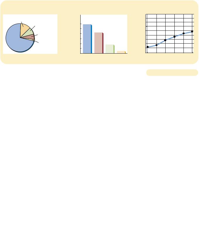
Three common graphs are shown in Figure 2A-1. The pie chart in panel (a) shows how total income in the United States is divided among the sources of income, including compensation of employees, corporate profits, and so on. A slice of the pie represents each source’s share of the total. The bar graph in panel (b) compares a measure of average income, called real GDP per person, for four countries. The height of each bar represents the average income in each country. The time-series graph in panel (c) traces the rising productivity in the U.S. business sector over time. The height of the line shows output per hour in each year. You have probably seen similar graphs presented in newspapers and magazines.

36

	CHAPTER 2	THINKING LIKE AN ECONOMIST	37
(a) Pie Chart	(b) Bar Graph	(c) Time-Series Graph

Corporate		Real GDP per	United		Productivity
			States
profits (12%)		Person in 1997			Index
			($28,740)
				United
	Proprietors’	30,000
	income (8%)	25,000	Kingdom
			($20,520)		115
	Interest	20,000
					95
	income (6%)			Mexico
		15,000			75
Compensation
	Rental	10,000		($8,120)	55
of employees
	income (2%)	5,000		India	35
(72%)				($1,950)
					0
		0
					1950 1960 1970 1980 1990 2000

TYPES OF GRAPHS. The pie chart in panel (a) shows how U.S. national income is derived		Figur e 2A-1
from various sources. The bar graph in panel (b) compares the average income in four
countries. The time-series graph in panel (c) shows the growth in productivity of the U.S.
business sector from 1950 to 2000.

GRAPHS OF TWO VARIABLES: THE COORDINATE SYSTEM

Although the three graphs in Figure 2A-1 are useful in showing how a variable changes over time or across individuals, such graphs are limited in how much they can tell us. These graphs display information only on a single variable. Economists are often concerned with the relationships between variables. Thus, they need to be able to display two variables on a single graph. The coordinate system makes this possible.

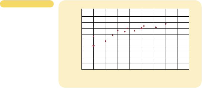
Suppose you want to examine the relationship between study time and grade point average. For each student in your class, you could record a pair of numbers: hours per week spent studying and grade point average. These numbers could then be placed in parentheses as an ordered pair and appear as a single point on the graph. Albert E., for instance, is represented by the ordered pair (25 hours/week, 3.5 GPA), while his “what-me-worry?” classmate Alfred E. is represented by the ordered pair (5 hours/week, 2.0 GPA).

We can graph these ordered pairs on a two-dimensional grid. The first number in each ordered pair, called the x-coordinate, tells us the horizontal location of the point. The second number, called the y-coordinate, tells us the vertical location of the point. The point with both an x-coordinate and a y-coordinate of zero is known as the origin. The two coordinates in the ordered pair tell us where the point is located in relation to the origin: x units to the right of the origin and y units above it.

Figure 2A-2 graphs grade point average against study time for Albert E., Alfred E., and their classmates. This type of graph is called a scatterplot because it plots scattered points. Looking at this graph, we immediately notice that points farther to the right (indicating more study time) also tend to be higher (indicating a better grade point average). Because study time and grade point average typically move in the same direction, we say that these two variables have a positive

38 PART ONE INTRODUCTION

Figur e 2A-2

USING THE COORDINATE SYSTEM.

Grade point average is measured on the vertical axis and study time on the horizontal axis. Albert E., Alfred E., and their classmates are represented by various points. We can see from the graph that students who study more tend to get higher grades.

Grade

Point

Average

	4.0
	3.5	Albert E.
	3.0
		(25, 3.5)

2.5

Alfred E.

2.0

(5, 2.0)

1.5

1.0

0.5

0	5	10	15	20	25	30	35	40 Study
								Time

(hours per week)

correlation. By contrast, if we were to graph party time and grades, we would likely find that higher party time is associated with lower grades; because these variables typically move in opposite directions, we would call this a negative correlation. In either case, the coordinate system makes the correlation between the two variables easy to see.

CURVES IN THE COORDINATE SYSTEM

Students who study more do tend to get higher grades, but other factors also influence a student’s grade. Previous preparation is an important factor, for instance, as are talent, attention from teachers, even eating a good breakfast. A scatterplot like Figure 2A-2 does not attempt to isolate the effect that study has on grades from the effects of other variables. Often, however, economists prefer looking at how one variable affects another holding everything else constant.

To see how this is done, let’s consider one of the most important graphs in eco- nomics—the demand curve. The demand curve traces out the effect of a good’s price on the quantity of the good consumers want to buy. Before showing a demand curve, however, consider Table 2A-1, which shows how the number of novels that Emma buys depends on her income and on the price of novels. When novels are cheap, Emma buys them in large quantities. As they become more expensive, she borrows books from the library instead of buying them or chooses to go to the movies instead of reading. Similarly, at any given price, Emma buys more novels when she has a higher income. That is, when her income increases, she spends part of the additional income on novels and part on other goods.

We now have three variables—the price of novels, income, and the number of novels purchased—which is more than we can represent in two dimensions. To

CHAPTER 2 THINKING LIKE AN ECONOMIST

39

		INCOME
PRICE	$20,000	$30,000	$40,000
$10	2 novels	5 novels	8 novels
9	6	9	12
8	10	13	16
7	14	17	20
6	18	21	24
5	22	25	28
	Demand	Demand	Demand
	curve, D3	curve, D1	curve, D2

Price of

Novels

$11

(5, $10)

10

9(9, $9)

8	(13, $8)
7	(17, $7)

(21, $6)

6

5						(25, $5)
4						Demand, D1
3
2
1
0	5	10	15	20	25	30	Quantity
							of Novels
							Purchased

put the information from Table 2A-1 in graphical form, we need to hold one of the three variables constant and trace out the relationship between the other two. Because the demand curve represents the relationship between price and quantity demanded, we hold Emma’s income constant and show how the number of novels she buys varies with the price of novels.

Suppose that Emma’s income is $30,000 per year. If we place the number of novels Emma purchases on the x-axis and the price of novels on the y-axis, we can

Table 2A-1

NOVELS PURCHASED BY EMMA.

This table shows the number of novels Emma buys at various incomes and prices. For any given level of income, the data on price and quantity demanded can be graphed to produce Emma’s demand curve for novels, as in Figure 2A-3.

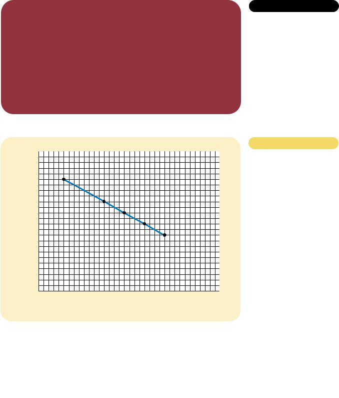
Figur e 2A-3

DEMAND CURVE. The line D1 shows how Emma’s purchases of novels depend on the price of novels when her income is held constant. Because the price and the quantity demanded are negatively related, the demand curve slopes downward.

40 PART ONE INTRODUCTION

graphically represent the middle column of Table 2A-1. When the points that represent these entries from the table—(5 novels, $10), (9 novels, $9), and so on—are connected, they form a line. This line, pictured in Figure 2A-3, is known as Emma’s demand curve for novels; it tells us how many novels Emma purchases at any given price. The demand curve is downward sloping, indicating that a higher price reduces the quantity of novels demanded. Because the quantity of novels demanded and the price move in opposite directions, we say that the two variables are negatively related. (Conversely, when two variables move in the same direction, the curve relating them is upward sloping, and we say the variables are positively related.)

Now suppose that Emma’s income rises to $40,000 per year. At any given price, Emma will purchase more novels than she did at her previous level of income. Just as earlier we drew Emma’s demand curve for novels using the entries from the middle column of Table 2A-1, we now draw a new demand curve using the entries from the right-hand column of the table. This new demand curve (curve D2) is pictured alongside the old one (curve D1) in Figure 2A-4; the new curve is a similar line drawn farther to the right. We therefore say that Emma’s demand curve for novels shifts to the right when her income increases. Likewise, if Emma’s income were to fall to $20,000 per year, she would buy fewer novels at any given price and her demand curve would shift to the left (to curve D3).

In economics, it is important to distinguish between movements along a curve and shifts of a curve. As we can see from Figure 2A-3, if Emma earns $30,000 per year and novels cost $8 apiece, she will purchase 13 novels per year. If the price of novels falls to $7, Emma will increase her purchases of novels to 17 per year. The demand curve, however, stays fixed in the same place. Emma still buys the same

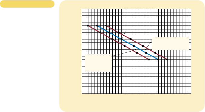
Figur e 2A-4

SHIFTING DEMAND CURVES.

The location of Emma’s demand curve for novels depends on how much income she earns. The more she earns, the more novels she will purchase at any given price, and the farther to the right her demand curve will lie. Curve D1 represents Emma’s original demand curve when her income is $30,000 per year. If her income rises to $40,000 per year, her demand curve shifts to D2. If her income falls to $20,000 per year, her demand curve shifts

to D3.

Price of

Novels

$11

10
9		(13, $8)
		(16, $8)
8
	(10, $8)	When income increases,
		the demand curve
7
		shifts to the right.

6
5	When income			D3
	decreases, the
				(income =	D1	D2 (income =
	demand curve
4				$20,000)	(income =	$40,000)
	shifts to the left.
					$30,000)
3
2
1
0	5	10	13 1516	20	25	30	Quantity
							of Novels
							Purchased

CHAPTER 2 THINKING LIKE AN ECONOMIST

41

number of novels at each price, but as the price falls she moves along her demand curve from left to right. By contrast, if the price of novels remains fixed at $8 but her income rises to $40,000, Emma increases her purchases of novels from 13 to 16 per year. Because Emma buys more novels at each price, her demand curve shifts out, as shown in Figure 2A-4.

There is a simple way to tell when it is necessary to shift a curve. When a variable that is not named on either axis changes, the curve shifts. Income is on neither the x-axis nor the y-axis of the graph, so when Emma’s income changes, her demand curve must shift. Any change that affects Emma’s purchasing habits besides a change in the price of novels will result in a shift in her demand curve. If, for instance, the public library closes and Emma must buy all the books she wants to read, she will demand more novels at each price, and her demand curve will shift to the right. Or, if the price of movies falls and Emma spends more time at the movies and less time reading, she will demand fewer novels at each price, and her demand curve will shift to the left. By contrast, when a variable on an axis of the graph changes, the curve does not shift. We read the change as a movement along the curve.

SLOPE

One question we might want to ask about Emma is how much her purchasing habits respond to price. Look at the demand curve pictured in Figure 2A-5. If this curve is very steep, Emma purchases nearly the same number of novels regardless

Price of

Novels

$11

10
9
8		(13, $8)
7	6	8 2
			(21, $6)
6
		21 13	8

5	Demand, D1
4

3

2

1

0

5

10

13

15

20 21

25

30

Quantity

of Novels

Purchased

Figur e 2A-5

CALCULATING THE SLOPE OF A

LINE. To calculate the slope of the demand curve, we can look at the changes in the x- and y-coordinates as we move from the point (21 novels, $6) to the point (13 novels, $8). The slope of the line is the ratio of the change in the y-coordinate ( 2) to the change in the x-coordinate ( 8), which equals 1/4.