Mankiw Principles of Macroeconomics (3rd ed)

134	PART TWO SUPPLY AND DEMAND I: HOW MARKETS WORK

the tax.) The difference in the two panels is the relative elasticity of supply and demand.

Panel (a) of Figure 6-9 shows a tax in a market with very elastic supply and relatively inelastic demand. That is, sellers are very responsive to the price of the good, whereas buyers are not very responsive. When a tax is imposed on a market with these elasticities, the price received by sellers does not fall much, so sellers bear only a small burden. By contrast, the price paid by buyers rises substantially, indicating that buyers bear most of the burden of the tax.

Panel (b) of Figure 6-9 shows a tax in a market with relatively inelastic supply and very elastic demand. In this case, sellers are not very responsive to the price, while buyers are very responsive. The figure shows that when a tax is imposed, the price paid by buyers does not rise much, while the price received by sellers falls substantially. Thus, sellers bear most of the burden of the tax.

The two panels of Figure 6-9 show a general lesson about how the burden of a tax is divided: A tax burden falls more heavily on the side of the market that is less elastic. Why is this true? In essence, the elasticity measures the willingness of buyers or sellers to leave the market when conditions become unfavorable. A small elasticity of demand means that buyers do not have good alternatives to consuming this particular good. A small elasticity of supply means that sellers do not have good alternatives to producing this particular good. When the good is taxed, the side of the market with fewer good alternatives cannot easily leave the market and must, therefore, bear more of the burden of the tax.

We can apply this logic to the payroll tax, which was discussed in the previous case study. Most labor economists believe that the supply of labor is much less elastic than the demand. This means that workers, rather than firms, bear most of the burden of the payroll tax. In other words, the distribution of the tax burden is not at all close to the fifty-fifty split that lawmakers intended.

“IF THIS BOAT WERE ANY MORE EXPENSIVE, WE WOULD BE PLAYING GOLF.”

CASE STUDY WHO PAYS THE LUXURY TAX?

In 1990, Congress adopted a new luxury tax on items such as yachts, private airplanes, furs, jewelry, and expensive cars. The goal of the tax was to raise revenue from those who could most easily afford to pay. Because only the rich could afford to buy such extravagances, taxing luxuries seemed a logical way of taxing the rich.

Yet, when the forces of supply and demand took over, the outcome was quite different from what Congress intended. Consider, for example, the market for yachts. The demand for yachts is quite elastic. A millionaire can easily not buy a yacht; she can use the money to buy a bigger house, take a European vacation, or leave a larger bequest to her heirs. By contrast, the supply of yachts is relatively inelastic, at least in the short run. Yacht factories are not easily converted to alternative uses, and workers who build yachts are not eager to change careers in response to changing market conditions.

Our analysis makes a clear prediction in this case. With elastic demand and inelastic supply, the burden of a tax falls largely on the suppliers. That is, a tax on yachts places a burden largely on the firms and workers who build yachts because they end up getting a lower price for their product. The workers, however, are not wealthy. Thus, the burden of a luxury tax falls more on the middle class than on the rich.

CHAPTER 6 SUPPLY, DEMAND, AND GOVERNMENT POLICIES

135

The mistaken assumptions about the incidence of the luxury tax quickly became apparent after the tax went into effect. Suppliers of luxuries made their congressional representatives well aware of the economic hardship they experienced, and Congress repealed most of the luxury tax in 1993.

QUICK QUIZ: In a supply-and-demand diagram, show how a tax on car buyers of $1,000 per car affects the quantity of cars sold and the price of cars. In another diagram, show how a tax on car sellers of $1,000 per car affects the quantity of cars sold and the price of cars. In both of your diagrams, show the change in the price paid by car buyers and the change in price received by car sellers.

CONCLUSION

The economy is governed by two kinds of laws: the laws of supply and demand and the laws enacted by governments. In this chapter we have begun to see how these laws interact. Price controls and taxes are common in various markets in the economy, and their effects are frequently debated in the press and among policymakers. Even a little bit of economic knowledge can go a long way toward understanding and evaluating these policies.

In subsequent chapters we will analyze many government policies in greater detail. We will examine the effects of taxation more fully, and we will consider a broader range of policies than we considered here. Yet the basic lessons of this chapter will not change: When analyzing government policies, supply and demand are the first and most

Summar y

A price ceiling is a legal maximum on the price of a good or service. An example is rent control. If the price ceiling is below the equilibrium price, the quantity demanded exceeds the quantity supplied. Because of the resulting shortage, sellers must in some way ration the good or service among buyers.

A price floor is a legal minimum on the price of a good or service. An example is the minimum wage. If the price floor is above the equilibrium price, the quantity supplied exceeds the quantity demanded. Because of the resulting surplus, buyers’ demands for the good or service must in some way be rationed among sellers.

When the government levies a tax on a good, the equilibrium quantity of the good falls. That is, a tax on a market shrinks the size of the market.

A tax on a good places a wedge between the price paid by buyers and the price received by sellers. When the market moves to the new equilibrium, buyers pay more for the good and sellers receive less for it. In this sense, buyers and sellers share the tax burden. The incidence of a tax does not depend on whether the tax is levied on buyers or sellers.

The incidence of a tax depends on the price elasticities of supply and demand. The burden tends to fall on the side of the market that is less elastic because that side of the market can respond less easily to the tax by changing the quantity bought or sold.

136 PART TWO SUPPLY AND DEMAND I: HOW MARKETS WORK

	Key Concepts
price ceiling, p. 118	incidence, p. 129
	Questions for Review

1.Give an example of a price ceiling price floor.

2.Which causes a shortage of a price floor? Which causes a

3.What mechanisms allocate good is not allowed to bring equilibrium?

4.Explain why economists usually prices.

between a tax paid by buyers and

a good affect the price paid by received by sellers, and the quantity

how the burden of a tax is divided sellers? Why?

Problems and Applications

1.Lovers of classical music persuade Congress to impose a price ceiling of $40 per ticket. Does this policy get more or fewer people to attend classical music concerts?

2.The government has decided that the free-market price of cheese is too low.

a.Suppose the government imposes a binding price floor in the cheese market. Use a supply-and- demand diagram to show the effect of this policy on the price of cheese and the quantity of cheese sold. Is there a shortage or surplus of cheese?

b.Farmers complain that the price floor has reduced their total revenue. Is this possible? Explain.

c.In response to farmers’ complaints, the government agrees to purchase all of the surplus cheese at the price floor. Compared to the basic price floor, who benefits from this new policy? Who loses?

3.A recent study found that the demand and supply schedules for Frisbees are as follows:

PRICE PER	QUANTITY	QUANTITY
FRISBEE	DEMANDED	SUPPLIED
$11	1 million	15 million
10	2	12
9	4	9
8	6	6
7	8	3
6	10	1

a.What are the equilibrium price and quantity of Frisbees?

b.Frisbee manufacturers persuade the government that Frisbee production improves scientists’ understanding of aerodynamics and thus is important for national security. A concerned Congress votes to impose a price floor $2 above the equilibrium price. What is the new market price? How many Frisbees are sold?

c.Irate college students march on Washington and demand a reduction in the price of Frisbees. An even more concerned Congress votes to repeal the price floor and impose a price ceiling $1 below the former price floor. What is the new market price? How many Frisbees are sold?

4.Suppose the federal government requires beer drinkers to pay a $2 tax on each case of beer purchased. (In fact, both the federal and state governments impose beer taxes of some sort.)

a.Draw a supply-and-demand diagram of the market for beer without the tax. Show the price paid by consumers, the price received by producers, and the quantity of beer sold. What is the difference between the price paid by consumers and the price received by producers?

b.Now draw a supply-and-demand diagram for the beer market with the tax. Show the price paid by consumers, the price received by producers, and

CHAPTER 6 SUPPLY, DEMAND, AND GOVERNMENT POLICIES

137

the quantity of beer sold. What is the difference between the price paid by consumers and the price received by producers? Has the quantity of beer sold increased or decreased?

5.A senator wants to raise tax revenue and make workers better off. A staff member proposes raising the payroll tax paid by firms and using part of the extra revenue to reduce the payroll tax paid by workers. Would this accomplish the senator’s goal?

6.If the government places a $500 tax on luxury cars, will the price paid by consumers rise by more than $500, less than $500, or exactly $500? Explain.

7.Congress and the president decide that the United States should reduce air pollution by reducing its use of gasoline. They impose a $0.50 tax for each gallon of gasoline sold.

a.Should they impose this tax on producers or consumers? Explain carefully using a supply-and- demand diagram.

b.If the demand for gasoline were more elastic, would this tax be more effective or less effective in reducing the quantity of gasoline consumed? Explain with both words and a diagram.

c.Are consumers of gasoline helped or hurt by this tax? Why?

d.Are workers in the oil industry helped or hurt by this tax? Why?

8.A case study in this chapter discusses the federal minimum-wage law.

a.Suppose the minimum wage is above the equilibrium wage in the market for unskilled labor. Using a supply-and-demand diagram of the market for unskilled labor, show the market wage, the number of workers who are employed, and the number of workers who are unemployed. Also show the total wage payments to unskilled workers.

b.Now suppose the secretary of labor proposes an increase in the minimum wage. What effect would this increase have on employment? Does the change in employment depend on the elasticity of demand, the elasticity of supply, both elasticities, or neither?

c.What effect would this increase in the minimum wage have on unemployment? Does the change in unemployment depend on the elasticity of demand, the elasticity of supply, both elasticities, or neither?

d.If the demand for unskilled labor were inelastic, would the proposed increase in the minimum wage raise or lower total wage payments to unskilled workers? Would your answer change if the demand for unskilled labor were elastic?

9.Consider the following policies, each of which is aimed at reducing violent crime by reducing the use of guns. Illustrate each of these proposed policies in a supply- and-demand diagram of the gun market.

a.a tax on gun buyers

b.a tax on gun sellers

c.a price floor on guns

d.a tax on ammunition

10.The U.S. government administers two programs that affect the market for cigarettes. Media campaigns and labeling requirements are aimed at making the public aware of the dangers of cigarette smoking. At the same time, the Department of Agriculture maintains a price support program for tobacco farmers, which raises the price of tobacco above the equilibrium price.

a.How do these two programs affect cigarette consumption? Use a graph of the cigarette market in your answer.

b.What is the combined effect of these two programs on the price of cigarettes?

c.Cigarettes are also heavily taxed. What effect does this tax have on cigarette consumption?

11.A subsidy is the opposite of a tax. With a $0.50 tax on the buyers of ice-cream cones, the government collects $0.50 for each cone purchased; with a $0.50 subsidy for the buyers of ice-cream cones, the government pays buyers $0.50 for each cone purchased.

a.Show the effect of a $0.50 per cone subsidy on the demand curve for ice-cream cones, the effective price paid by consumers, the effective price received by sellers, and the quantity of cones sold.

b.Do consumers gain or lose from this policy? Do producers gain or lose? Does the government gain or lose?

C O N S U M E R S , P R O D U C E R S ,

A N D T H E E F F I C I E N C Y

O F M A R K E T S

When consumers go to grocery stores to buy their turkeys for Thanksgiving dinner, they may be disappointed that the price of turkey is as high as it is. At the same time, when farmers bring to market the turkeys they have raised, they wish the price of turkey were even higher. These views are not surprising: Buyers always want to pay less, and sellers always want to get paid more. But is there a “right price” for turkey from the standpoint of society as a whole?

In previous chapters we saw how, in market economies, the forces of supply and demand determine the prices of goods and services and the quantities sold. So far, however, we have described the way markets allocate scarce resources without directly addressing the question of whether these market allocations are desirable. In other words, our analysis has been positive (what is) rather than normative (what

IN THIS CHAPTER YOU WILL . . .

Examine the link between buyers’ willingness to pay for a good and the demand cur ve

Lear n how to define and measur e consumer surplus

Examine the link between sellers’ costs of pr oducing a good and the supply cur ve

Lear n how to define and measur e

pr oducer surplus

See that the equilibrium of supply and demand maximizes total surplus in a market

141

142	PART THREE SUPPLY AND DEMAND II: MARKETS AND WELFARE

should be). We know that the price of turkey adjusts to ensure that the quantity of turkey supplied equals the quantity of turkey demanded. But, at this equilibrium, is the quantity of turkey produced and consumed too small, too large, or just right?

welfar e economics In this chapter we take up the topic of welfare economics, the study of how the study of how the allocation of the allocation of resources affects economic well-being. We begin by examining the resources affects economic well-being benefits that buyers and sellers receive from taking part in a market. We then examine how society can make these benefits as large as possible. This analysis leads to a profound conclusion: The equilibrium of supply and demand in a market

maximizes the total benefits received by buyers and sellers.

As you may recall from Chapter 1, one of the Ten Principles of Economics is that markets are usually a good way to organize economic activity. The study of welfare economics explains this principle more fully. It also answers our question about the right price of turkey: The price that balances the supply and demand for turkey is, in a particular sense, the best one because it maximizes the total welfare of turkey consumers and turkey producers.

CONSUMER SURPLUS

willingness to pay

the maximum amount that a buyer will pay for a good

Table 7-1

FOUR POSSIBLE BUYERS’

WILLINGNESS TO PAY

We begin our study of welfare economics by looking at the benefits buyers receive from participating in a market.

WILLINGNESS TO PAY

Imagine that you own a mint-condition recording of Elvis Presley’s first album. Because you are not an Elvis Presley fan, you decide to sell it. One way to do so is to hold an auction.

Four Elvis fans show up for your auction: John, Paul, George, and Ringo. Each of them would like to own the album, but there is a limit to the amount that each is willing to pay for it. Table 7-1 shows the maximum price that each of the four possible buyers would pay. Each buyer’s maximum is called his willingness to pay, and it measures how much that buyer values the good. Each buyer would be eager to buy the album at a price less than his willingness to pay, would refuse to

BUYER	WILLINGNESS TO PAY
John	$100
Paul	80
George	70
Ringo	50

CHAPTER 7 CONSUMERS, PRODUCERS, AND THE EFFICIENCY OF MARKETS

143

buy the album at a price more than his willingness to pay, and would be indifferent about buying the album at a price exactly equal to his willingness to pay.

To sell your album, you begin the bidding at a low price, say $10. Because all four buyers are willing to pay much more, the price rises quickly. The bidding stops when John bids $80 (or slightly more). At this point, Paul, George, and Ringo have dropped out of the bidding, because they are unwilling to bid any more than $80. John pays you $80 and gets the album. Note that the album has gone to the buyer who values the album most highly.

What benefit does John receive from buying the Elvis Presley album? In a sense, John has found a real bargain: He is willing to pay $100 for the album but pays only $80 for it. We say that John receives consumer surplus of $20. Consumer surplus is the amount a buyer is willing to pay for a good minus the amount the buyer actually pays for it.

Consumer surplus measures the benefit to buyers of participating in a market. In this example, John receives a $20 benefit from participating in the auction because he pays only $80 for a good he values at $100. Paul, George, and Ringo get no consumer surplus from participating in the auction, because they left without the album and without paying anything.

Now consider a somewhat different example. Suppose that you had two identical Elvis Presley albums to sell. Again, you auction them off to the four possible buyers. To keep things simple, we assume that both albums are to be sold for the same price and that no buyer is interested in buying more than one album. Therefore, the price rises until two buyers are left.

In this case, the bidding stops when John and Paul bid $70 (or slightly higher). At this price, John and Paul are each happy to buy an album, and George and Ringo are not willing to bid any higher. John and Paul each receive consumer surplus equal to his willingness to pay minus the price. John’s consumer surplus is $30, and Paul’s is $10. John’s consumer surplus is higher now than it was previously, because he gets the same album but pays less for it. The total consumer surplus in the market is $40.

USING THE DEMAND CURVE TO MEASURE

CONSUMER SURPLUS

Consumer surplus is closely related to the demand curve for a product. To see how they are related, let’s continue our example and consider the demand curve for this rare Elvis Presley album.

We begin by using the willingness to pay of the four possible buyers to find the demand schedule for the album. Table 7-2 shows the demand schedule that corresponds to Table 7-1. If the price is above $100, the quantity demanded in the market is 0, because no buyer is willing to pay that much. If the price is between $80 and $100, the quantity demanded is 1, because only John is willing to pay such a high price. If the price is between $70 and $80, the quantity demanded is 2, because both John and Paul are willing to pay the price. We can continue this analysis for other prices as well. In this way, the demand schedule is derived from the willingness to pay of the four possible buyers.

Figure 7-1 graphs the demand curve that corresponds to this demand schedule. Note the relationship between the height of the demand curve and the buyers’ willingness to pay. At any quantity, the price given by the demand curve shows

consumer surplus

a buyer’s willingness to pay minus the amount the buyer actually pays

144	PART THREE SUPPLY AND DEMAND II: MARKETS AND WELFARE

Table 7-2

THE DEMAND SCHEDULE FOR THE

BUYERS IN TABLE 7-1

Figur e 7-1

THE DEMAND CURVE. This

figure graphs the demand curve from the demand schedule in Table 7-2. Note that the height of the demand curve reflects buyers’ willingness to pay.

PRICE	BUYERS	QUANTITY DEMANDED
More than $100	None	0
$80 to $100	John	1
$70 to $80	John, Paul	2
$50 to $70	John, Paul, George	3
$50 or less	John, Paul, George, Ringo	4

Price of

Album

$100 John’s willingness to pay

80							Paul’s willingness to pay
70
										George’s willingness to pay
50
													Ringo’s willingness to pay
													Demand
0	1			2		3				4				Quantity of
														Albums

the willingness to pay of the marginal buyer, the buyer who would leave the market first if the price were any higher. At a quantity of 4 albums, for instance, the demand curve has a height of $50, the price that Ringo (the marginal buyer) is willing to pay for an album. At a quantity of 3 albums, the demand curve has a height of $70, the price that George (who is now the marginal buyer) is willing to pay.

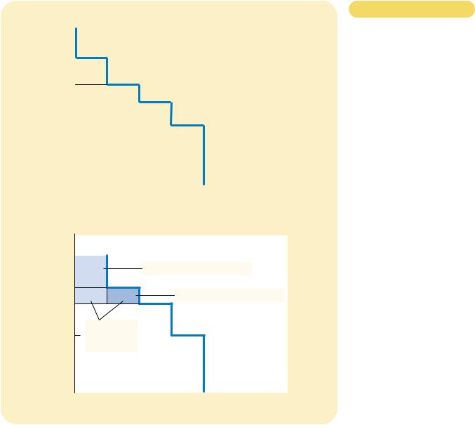
Because the demand curve reflects buyers’ willingness to pay, we can also use it to measure consumer surplus. Figure 7-2 uses the demand curve to compute consumer surplus in our example. In panel (a), the price is $80 (or slightly above), and the quantity demanded is 1. Note that the area above the price and below the demand curve equals $20. This amount is exactly the consumer surplus we computed earlier when only 1 album is sold.

Panel (b) of Figure 7-2 shows consumer surplus when the price is $70 (or slightly above). In this case, the area above the price and below the demand curve

CHAPTER 7 CONSUMERS, PRODUCERS, AND THE EFFICIENCY OF MARKETS

145

(a) Price = $80

Price of
Album
$100
							John’s consumer surplus ($20)
80
70
50										Demand
0	1				2		3		4		Quantity of
												Albums
							(b) Price = $70
Price of
Album
$100

John’s consumer surplus ($30)

80

Paul’s consumer surplus ($10)

70

Total

50consumer surplus ($40)

									Demand
0	1		2		3		4		Quantity of
									Albums

Figur e 7-2

MEASURING CONSUMER SURPLUS

WITH THE DEMAND CURVE. In

panel (a), the price of the good is $80, and the consumer surplus is $20. In panel (b), the price of the good is $70, and the consumer surplus is $40.

equals the total area of the two rectangles: John’s consumer surplus at this price is $30 and Paul’s is $10. This area equals a total of $40. Once again, this amount is the consumer surplus we computed earlier.

The lesson from this example holds for all demand curves: The area below the demand curve and above the price measures the consumer surplus in a market. The reason is that the height of the demand curve measures the value buyers place on the good, as measured by their willingness to pay for it. The difference between this willingness to pay and the market price is each buyer’s consumer surplus. Thus, the total area below the demand curve and above the price is the sum of the consumer surplus of all buyers in the market for a good or service.