Mankiw Principles of Macroeconomics (3rd ed)

42 PART ONE INTRODUCTION

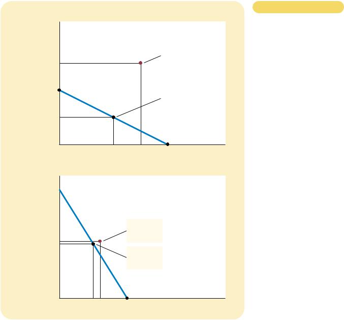
of whether they are cheap or expensive. If this curve is much flatter, Emma purchases many fewer novels when the price rises. To answer questions about how much one variable responds to changes in another variable, we can use the concept of slope.

The slope of a line is the ratio of the vertical distance covered to the horizontal distance covered as we move along the line. This definition is usually written out in mathematical symbols as follows:

y slope = x ,

where the Greek letter ∆ (delta) stands for the change in a variable. In other words, the slope of a line is equal to the “rise” (change in y) divided by the “run” (change in x). The slope will be a small positive number for a fairly flat upward-sloping line, a large positive number for a steep upward-sloping line, and a negative number for a downward-sloping line. A horizontal line has a slope of zero because in this case the y-variable never changes; a vertical line is defined to have an infinite slope because the y-variable can take any value without the x-variable changing at all.

What is the slope of Emma’s demand curve for novels? First of all, because the curve slopes down, we know the slope will be negative. To calculate a numerical value for the slope, we must choose two points on the line. With Emma’s income at $30,000, she will purchase 21 novels at a price of $6 or 13 novels at a price of $8. When we apply the slope formula, we are concerned with the change between these two points; in other words, we are concerned with the difference between them, which lets us know that we will have to subtract one set of values from the other, as follows:

	y		first y-coordinate second y-coordinate	6 8			2	1
slope =		=		=		=		=		.
	x		first x-coordinate second x-coordinate		21 13		8		4

Figure 2A-5 shows graphically how this calculation works. Try computing the slope of Emma’s demand curve using two different points. You should get exactly the same result, 1/4. One of the properties of a straight line is that it has the same slope everywhere. This is not true of other types of curves, which are steeper in some places than in others.

The slope of Emma’s demand curve tells us something about how responsive her purchases are to changes in the price. A small slope (a number close to zero) means that Emma’s demand curve is relatively flat; in this case, she adjusts the number of novels she buys substantially in response to a price change. A larger slope (a number farther from zero) means that Emma’s demand curve is relatively steep; in this case, she adjusts the number of novels she buys only slightly in response to a price change.

CAUSE AND EFFECT

Economists often use graphs to advance an argument about how the economy works. In other words, they use graphs to argue about how one set of events causes another set of events. With a graph like the demand curve, there is no doubt about cause and effect. Because we are varying price and holding all other

CHAPTER 2 THINKING LIKE AN ECONOMIST

43

variables constant, we know that changes in the price of novels cause changes in the quantity Emma demands. Remember, however, that our demand curve came from a hypothetical example. When graphing data from the real world, it is often more difficult to establish how one variable affects another.

The first problem is that it is difficult to hold everything else constant when measuring how one variable affects another. If we are not able to hold variables constant, we might decide that one variable on our graph is causing changes in the other variable when actually those changes are caused by a third omitted variable not pictured on the graph. Even if we have identified the correct two variables to look at, we might run into a second problem—reverse causality. In other words, we might decide that A causes B when in fact B causes A. The omitted-variable and reverse-causality traps require us to proceed with caution when using graphs to draw conclusions about causes and effects.

Omitted Variables To see how omitting a variable can lead to a deceptive graph, let’s consider an example. Imagine that the government, spurred by public concern about the large number of deaths from cancer, commissions an exhaustive study from Big Brother Statistical Services, Inc. Big Brother examines many of the items found in people’s homes to see which of them are associated with the risk of cancer. Big Brother reports a strong relationship between two variables: the number of cigarette lighters that a household owns and the probability that someone in the household will develop cancer. Figure 2A-6 shows this relationship.

What should we make of this result? Big Brother advises a quick policy response. It recommends that the government discourage the ownership of cigarette lighters by taxing their sale. It also recommends that the government require warning labels: “Big Brother has determined that this lighter is dangerous to your health.”

In judging the validity of Big Brother’s analysis, one question is paramount: Has Big Brother held constant every relevant variable except the one under consideration? If the answer is no, the results are suspect. An easy explanation for Figure 2A-6 is that people who own more cigarette lighters are more likely to smoke cigarettes and that cigarettes, not lighters, cause cancer. If Figure 2A-6 does not

Risk of

Cancer

0

Figur e 2A-6

GRAPH WITH AN OMITTED

VARIABLE. The upward-sloping curve shows that members of households with more cigarette lighters are more likely to develop cancer. Yet we should not conclude that ownership of lighters causes cancer because the

graph does not take into account

Number of Lighters in House

the number of cigarettes smoked.

44 PART ONE INTRODUCTION

hold constant the amount of smoking, it does not tell us the true effect of owning a cigarette lighter.

This story illustrates an important principle: When you see a graph being used to support an argument about cause and effect, it is important to ask whether the movements of an omitted variable could explain the results you see.

Reverse Causality Economists can also make mistakes about causality by misreading its direction. To see how this is possible, suppose the Association of American Anarchists commissions a study of crime in America and arrives at Figure 2A-7, which plots the number of violent crimes per thousand people in major cities against the number of police officers per thousand people. The anarchists note the curve’s upward slope and argue that because police increase rather than decrease the amount of urban violence, law enforcement should be abolished.

If we could run a controlled experiment, we would avoid the danger of reverse causality. To run an experiment, we would set the number of police officers in different cities randomly and then examine the correlation between police and crime. Figure 2A-7, however, is not based on such an experiment. We simply observe that more dangerous cities have more police officers. The explanation for this may be that more dangerous cities hire more police. In other words, rather than police causing crime, crime may cause police. Nothing in the graph itself allows us to establish the direction of causality.

It might seem that an easy way to determine the direction of causality is to examine which variable moves first. If we see crime increase and then the police force expand, we reach one conclusion. If we see the police force expand and then crime increase, we reach the other. Yet there is also a flaw with this approach: Often people change their behavior not in response to a change in their present conditions but in response to a change in their expectations of future conditions. A city that expects a major crime wave in the future, for instance, might well hire more police now. This problem is even easier to see in the case of babies and minivans. Couples often buy a minivan in anticipation of the birth of a child. The

Figur e 2A-7

GRAPH SUGGESTING REVERSE

CAUSALITY. The upwardsloping curve shows that cities with a higher concentration of police are more dangerous. Yet the graph does not tell us whether police cause crime or crime-plagued cities hire more police.

Violent

Crimes (per 1,000 people)

0	Police Officers

(per 1,000 people)

CHAPTER 2 THINKING LIKE AN ECONOMIST

45

minivan comes before the baby, but we wouldn’t want to conclude that the sale of minivans causes the population to grow!

There is no complete set of rules that says when it is appropriate to draw causal conclusions from graphs. Yet just keeping in mind that cigarette lighters don’t cause cancer (omitted variable) and minivans don’t cause larger families (reverse causality) will keep you from falling for many faulty economic arguments.

I N T E R D E P E N D E N C E A N D T H E

G A I N S F R O M T R A D E

Consider your typical day. You wake up in the morning, and you pour yourself juice from oranges grown in Florida and coffee from beans grown in Brazil. Over breakfast, you watch a news program broadcast from New York on your television made in Japan. You get dressed in clothes made of cotton grown in Georgia and sewn in factories in Thailand. You drive to class in a car made of parts manufactured in more than a dozen countries around the world. Then you open up your economics textbook written by an author living in Massachusetts, published by a company located in Texas, and printed on paper made from trees grown in Oregon.

Every day you rely on many people from around the world, most of whom you do not know, to provide you with the goods and services that you enjoy. Such interdependence is possible because people trade with one another. Those people who provide you with goods and services are not acting out of generosity or concern for your welfare. Nor is some government agency directing them to make what you

IN THIS CHAPTER YOU WILL . . .

Consider how ever yone can benefit

when people trade with one another

Learn the meaning of absolute advantage and comparative advantage

See how comparative advantage explains the gains fr om trade

Apply the theor y of comparative advantage to

ever yday life and national policy

47

48 PART ONE INTRODUCTION

want and to give it to you. Instead, people provide you and other consumers with the goods and services they produce because they get something in return.

In subsequent chapters we will examine how our economy coordinates the activities of millions of people with varying tastes and abilities. As a starting point for this analysis, here we consider the reasons for economic interdependence. One of the Ten Principles of Economics highlighted in Chapter 1 is that trade can make everyone better off. This principle explains why people trade with their neighbors and why nations trade with other nations. In this chapter we examine this principle more closely. What exactly do people gain when they trade with one another? Why do people choose to become interdependent?

A PARABLE FOR THE MODERN ECONOMY

To understand why people choose to depend on others for goods and services and how this choice improves their lives, let’s look at a simple economy. Imagine that there are two goods in the world—meat and potatoes. And there are two people in the world—a cattle rancher and a potato farmer—each of whom would like to eat both meat and potatoes.

The gains from trade are most obvious if the rancher can produce only meat and the farmer can produce only potatoes. In one scenario, the rancher and the farmer could choose to have nothing to do with each other. But after several months of eating beef roasted, boiled, broiled, and grilled, the rancher might decide that self-sufficiency is not all it’s cracked up to be. The farmer, who has been eating potatoes mashed, fried, baked, and scalloped, would likely agree. It is easy to see that trade would allow them to enjoy greater variety: Each could then have a hamburger with french fries.

Although this scene illustrates most simply how everyone can benefit from trade, the gains would be similar if the rancher and the farmer were each capable of producing the other good, but only at great cost. Suppose, for example, that the potato farmer is able to raise cattle and produce meat, but that he is not very good at it. Similarly, suppose that the cattle rancher is able to grow potatoes, but that her land is not very well suited for it. In this case, it is easy to see that the farmer and the rancher can each benefit by specializing in what he or she does best and then trading with the other.

The gains from trade are less obvious, however, when one person is better at producing every good. For example, suppose that the rancher is better at raising cattle and better at growing potatoes than the farmer. In this case, should the rancher or farmer choose to remain self-sufficient? Or is there still reason for them to trade with each other? To answer this question, we need to look more closely at the factors that affect such a decision.

PRODUCTION POSSIBILITIES

Suppose that the farmer and the rancher each work 40 hours a week and can devote this time to growing potatoes, raising cattle, or a combination of the two. Table 3-1 shows the amount of time each person requires to produce 1 pound of

CHAPTER 3 INTERDEPENDENCE AND THE GAINS FROM TRADE

49

							Table 3-1
	HOURS NEEDED TO			AMOUNT PRODUCED
							THE PRODUCTION
	MAKE 1 POUND OF:				IN 40 HOURS
							OPPORTUNITIES OF THE
	MEAT	POTATOES		MEAT	POTATOES		FARMER AND THE RANCHER
FARMER	20 hours/lb	10 hours/lb		2 lbs	4 lbs
RANCHER	1 hour/lb	8 hours/lb		40 lbs	5 lbs

Figur e 3-1

(a) The Farmer’s Production Possibilities Frontier

Meat (pounds)				THE PRODUCTION POSSIBILITIES
				FRONTIER. Panel (a) shows the
				combinations of meat and
				potatoes that the farmer can
				produce. Panel (b) shows the
				combinations of meat and
				potatoes that the rancher can
				produce. Both production
2				possibilities frontiers are derived
				from Table 3-1 and the
				assumption that the farmer and
1		A		rancher each work 40 hours per
				week.
0	2	4	Potatoes (pounds)
	(b) The Rancher’s Production Possibilities Frontier
Meat (pounds)
40

20

0

2 1/2

5

Potatoes (pounds)

50 PART ONE INTRODUCTION

each good. The farmer can produce a pound of potatoes in 10 hours and a pound of meat in 20 hours. The rancher, who is more productive in both activities, can produce a pound of potatoes in 8 hours and a pound of meat in 1 hour.

Panel (a) of Figure 3-1 illustrates the amounts of meat and potatoes that the farmer can produce. If the farmer devotes all 40 hours of his time to potatoes, he produces 4 pounds of potatoes and no meat. If he devotes all his time to meat, he produces 2 pounds of meat and no potatoes. If the farmer divides his time equally between the two activities, spending 20 hours on each, he produces 2 pounds of potatoes and 1 pound of meat. The figure shows these three possible outcomes and all others in between.

This graph is the farmer’s production possibilities frontier. As we discussed in Chapter 2, a production possibilities frontier shows the various mixes of output that an economy can produce. It illustrates one of the Ten Principles of Economics in Chapter 1: People face tradeoffs. Here the farmer faces a tradeoff between producing meat and producing potatoes. You may recall that the production possibilities frontier in Chapter 2 was drawn bowed out; in this case, the tradeoff between the two goods depends on the amounts being produced. Here, however, the farmer’s technology for producing meat and potatoes (as summarized in Table 3-1) allows him to switch between one good and the other at a constant rate. In this case, the production possibilities frontier is a straight line.

Panel (b) of Figure 3-1 shows the production possibilities frontier for the rancher. If the rancher devotes all 40 hours of her time to potatoes, she produces 5 pounds of potatoes and no meat. If she devotes all her time to meat, she produces 40 pounds of meat and no potatoes. If the rancher divides her time equally, spending 20 hours on each activity, she produces 2 1/2 pounds of potatoes and 20 pounds of meat. Once again, the production possibilities frontier shows all the possible outcomes.

If the farmer and rancher choose to be self-sufficient, rather than trade with each other, then each consumes exactly what he or she produces. In this case, the production possibilities frontier is also the consumption possibilities frontier. That is, without trade, Figure 3-1 shows the possible combinations of meat and potatoes that the farmer and rancher can each consume.

Although these production possibilities frontiers are useful in showing the tradeoffs that the farmer and rancher face, they do not tell us what the farmer and rancher will actually choose to do. To determine their choices, we need to know the tastes of the farmer and the rancher. Let’s suppose they choose the combinations identified by points A and B in Figure 3-1: The farmer produces and consumes 2 pounds of potatoes and 1 pound of meat, while the rancher produces and consumes 2 1/2 pounds of potatoes and 20 pounds of meat.

SPECIALIZATION AND TRADE

After several years of eating combination B, the rancher gets an idea and goes to talk to the farmer:

RANCHER: Farmer, my friend, have I got a deal for you! I know how to improve life for both of us. I think you should stop producing meat altogether and devote all your time to growing potatoes. According to my calculations, if you work 40 hours a week growing potatoes, you’ll

CHAPTER 3 INTERDEPENDENCE AND THE GAINS FROM TRADE

51

(a) How Trade Increases the Farmer’s Consumption

Meat (pounds)

			Farmer’s
		A*	consumption
	3		with trade
	2
			Farmer’s
			consumption
			without trade

A

1

0

2

3

4

Potatoes (pounds)

(b) How Trade Increases the Rancher’s Consumption

Meat (pounds)

40

		Rancher’s
	B*	consumption
21		with trade
20	B
		Rancher’s
		consumption
		without trade

Figur e 3-2

HOW TRADE EXPANDS THE

SET OF CONSUMPTION

OPPORTUNITIES. The proposed trade between the farmer and the rancher offers each of them a combination of meat and potatoes that would be impossible in the absence of trade. In panel (a), the farmer gets to consume at point A* rather than point A. In panel (b), the rancher gets to consume at point B* rather than point B. Trade allows each to consume more meat and more potatoes.

0

2 1/2 3

5

Potatoes (pounds)

produce 4 pounds of potatoes. If you give me 1 of those 4 pounds, I’ll give you 3 pounds of meat in return. In the end, you’ll get to eat 3 pounds of potatoes and 3 pounds of meat every week, instead of the 2 pounds of potatoes and 1 pound of meat you now get. If you go along with my plan, you’ll have more of both foods. [To illustrate her point, the rancher shows the farmer panel (a) of Figure 3-2.]

FARMER: (sounding skeptical) That seems like a good deal for me. But I don’t understand why you are offering it. If the deal is so good for me, it can’t be good for you too.