Mankiw Principles of Macroeconomics (3rd ed)

146	PART THREE SUPPLY AND DEMAND II: MARKETS AND WELFARE

HOW A LOWER PRICE RAISES CONSUMER SURPLUS

Because buyers always want to pay less for the goods they buy, a lower price makes buyers of a good better off. But how much does buyers’ well-being rise in response to a lower price? We can use the concept of consumer surplus to answer this question precisely.

Figure 7-3 shows a typical downward-sloping demand curve. Although this demand curve appears somewhat different in shape from the steplike demand curves in our previous two figures, the ideas we have just developed apply nonetheless: Consumer surplus is the area above the price and below the demand curve. In panel (a), consumer surplus at a price of P1 is the area of triangle ABC.

Figur e 7-3

HOW THE PRICE AFFECTS CONSUMER SURPLUS. In panel

(a), the price is P1, the quantity demanded is Q1, and consumer surplus equals the area of the triangle ABC. When the price falls from P1 to P2, as in panel (b), the quantity demanded rises from Q1 to Q2, and the consumer surplus rises to the area of the triangle ADF. The increase in consumer surplus (area BCFD) occurs in part because existing consumers now pay less (area BCED) and in part because new consumers enter the market at the lower price (area CEF).

(a) Consumer Surplus at Price P1

Price

A

Consumer

surplus

P1

B

C

Demand

0

Q1

Quantity

(b) Consumer Surplus at Price P2

Price

A

		Initial
		consumer
		surplus
P1						Consumer surplus
		B				to new consumers
P2
		D		E
		Additional consumer				Demand
		surplus to initial
		consumers
0			Q1		Q2		Quantity

CHAPTER 7 CONSUMERS, PRODUCERS, AND THE EFFICIENCY OF MARKETS

147

Now suppose that the price falls from P1 to P2, as shown in panel (b). The consumer surplus now equals area ADF. The increase in consumer surplus attributable to the lower price is the area BCFD.

This increase in consumer surplus is composed of two parts. First, those buyers who were already buying Q1 of the good at the higher price P1 are better off because they now pay less. The increase in consumer surplus of existing buyers is the reduction in the amount they pay; it equals the area of the rectangle BCED. Second, some new buyers enter the market because they are now willing to buy the good at the lower price. As a result, the quantity demanded in the market increases from Q1 to Q2. The consumer surplus these newcomers receive is the area of the triangle CEF.

WHAT DOES CONSUMER SURPLUS MEASURE?

Our goal in developing the concept of consumer surplus is to make normative judgments about the desirability of market outcomes. Now that you have seen what consumer surplus is, let’s consider whether it is a good measure of economic well-being.

Imagine that you are a policymaker trying to design a good economic system. Would you care about the amount of consumer surplus? Consumer surplus, the amount that buyers are willing to pay for a good minus the amount they actually pay for it, measures the benefit that buyers receive from a good as the buyers themselves perceive it. Thus, consumer surplus is a good measure of economic well-being if policymakers want to respect the preferences of buyers.

In some circumstances, policymakers might choose not to care about consumer surplus because they do not respect the preferences that drive buyer behavior. For example, drug addicts are willing to pay a high price for heroin. Yet we would not say that addicts get a large benefit from being able to buy heroin at a low price (even though addicts might say they do). From the standpoint of society, willingness to pay in this instance is not a good measure of the buyers’ benefit, and consumer surplus is not a good measure of economic well-being, because addicts are not looking after their own best interests.

In most markets, however, consumer surplus does reflect economic wellbeing. Economists normally presume that buyers are rational when they make decisions and that their preferences should be respected. In this case, consumers are the best judges of how much benefit they receive from the goods they buy.

QUICK QUIZ: Draw a demand curve for turkey. In your diagram, show a price of turkey and the consumer surplus that results from that price. Explain in words what this consumer surplus measures.

PRODUCER SURPLUS

We now turn to the other side of the market and consider the benefits sellers receive from participating in a market. As you will see, our analysis of sellers’ welfare is similar to our analysis of buyers’ welfare.

148	PART THREE SUPPLY AND DEMAND II: MARKETS AND WELFARE

cost

the value of everything a seller must give up to produce a good

producer surplus

the amount a seller is paid for a good minus the seller’s cost

Table 7-3

THE COSTS OF FOUR POSSIBLE

SELLERS

COST AND THE WILLINGNESS TO SELL

Imagine now that you are a homeowner, and you need to get your house painted. You turn to four sellers of painting services: Mary, Frida, Georgia, and Grandma. Each painter is willing to do the work for you if the price is right. You decide to take bids from the four painters and auction off the job to the painter who will do the work for the lowest price.

Each painter is willing to take the job if the price she would receive exceeds her cost of doing the work. Here the term cost should be interpreted as the painters’ opportunity cost: It includes the painters’ out-of-pocket expenses (for paint, brushes, and so on) as well as the value that the painters place on their own time. Table 7-3 shows each painter’s cost. Because a painter’s cost is the lowest price she would accept for her work, cost is a measure of her willingness to sell her services. Each painter would be eager to sell her services at a price greater than her cost, would refuse to sell her services at a price less than her cost, and would be indifferent about selling her services at a price exactly equal to her cost.

When you take bids from the painters, the price might start off high, but it quickly falls as the painters compete for the job. Once Grandma has bid $600 (or slightly less), she is the sole remaining bidder. Grandma is happy to do the job for this price, because her cost is only $500. Mary, Frida, and Georgia are unwilling to do the job for less than $600. Note that the job goes to the painter who can do the work at the lowest cost.

What benefit does Grandma receive from getting the job? Because she is willing to do the work for $500 but gets $600 for doing it, we say that she receives producer surplus of $100. Producer surplus is the amount a seller is paid minus the cost of production. Producer surplus measures the benefit to sellers of participating in a market.

Now consider a somewhat different example. Suppose that you have two houses that need painting. Again, you auction off the jobs to the four painters. To keep things simple, let’s assume that no painter is able to paint both houses and that you will pay the same amount to paint each house. Therefore, the price falls until two painters are left.

In this case, the bidding stops when Georgia and Grandma each offer to do the job for a price of $800 (or slightly less). At this price, Georgia and Grandma are willing to do the work, and Mary and Frida are not willing to bid a lower price. At a price of $800, Grandma receives producer surplus of $300, and Georgia receives producer surplus of $200. The total producer surplus in the market is $500.

SELLER	COST
Mary	$900
Frida	800
Georgia	600
Grandma	500

CHAPTER 7 CONSUMERS, PRODUCERS, AND THE EFFICIENCY OF MARKETS

149

USING THE SUPPLY CURVE TO MEASURE

PRODUCER SURPLUS

Just as consumer surplus is closely related to the demand curve, producer surplus is closely related to the supply curve. To see how, let’s continue our example.

We begin by using the costs of the four painters to find the supply schedule for painting services. Table 7-4 shows the supply schedule that corresponds to the costs in Table 7-3. If the price is below $500, none of the four painters is willing to do the job, so the quantity supplied is zero. If the price is between $500 and $600, only Grandma is willing to do the job, so the quantity supplied is 1. If the price is between $600 and $800, Grandma and Georgia are willing to do the job, so the quantity supplied is 2, and so on. Thus, the supply schedule is derived from the costs of the four painters.

Figure 7-4 graphs the supply curve that corresponds to this supply schedule. Note that the height of the supply curve is related to the sellers’ costs. At any quantity, the price given by the supply curve shows the cost of the marginal seller, the

PRICE	SELLERS	QUANTITY SUPPLIED
$900 or more	Mary, Frida, Georgia, Grandma	4
$800 to $900	Frida, Georgia, Grandma	3
$600 to $800	Georgia, Grandma	2
$500 to $600	Grandma	1
Less than $500	None	0

Table 7-4

THE SUPPLY SCHEDULE FOR THE

SELLERS IN TABLE 7-3

Figur e 7-4

Price of

Supply

House

Painting

$900

Mary’s cost

800

Frida’s cost

600

Georgia’s cost

500

Grandma’s cost

THE SUPPLY CURVE. This figure graphs the supply curve from the supply schedule in Table 7-4.

Note that the height of the supply curve reflects sellers’ costs.

0	1	2	3	4	Quantity of
					Houses Painted

150	PART THREE SUPPLY AND DEMAND II: MARKETS AND WELFARE

seller who would leave the market first if the price were any lower. At a quantity of 4 houses, for instance, the supply curve has a height of $900, the cost that Mary (the marginal seller) incurs to provide her painting services. At a quantity of 3 houses, the supply curve has a height of $800, the cost that Frida (who is now the marginal seller) incurs.

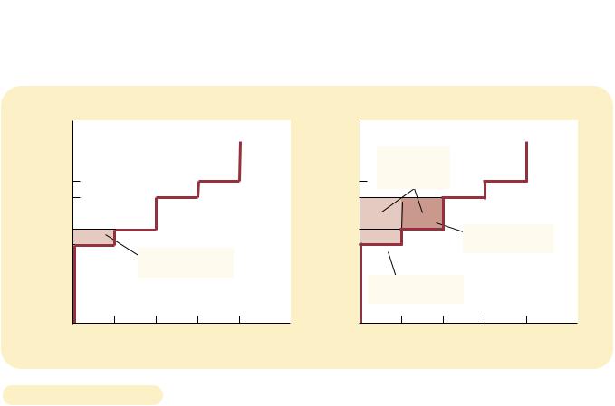
Because the supply curve reflects sellers’ costs, we can use it to measure producer surplus. Figure 7-5 uses the supply curve to compute producer surplus in our example. In panel (a), we assume that the price is $600. In this case, the quantity supplied is 1. Note that the area below the price and above the supply curve equals $100. This amount is exactly the producer surplus we computed earlier for Grandma.

Panel (b) of Figure 7-5 shows producer surplus at a price of $800. In this case, the area below the price and above the supply curve equals the total area of the two rectangles. This area equals $500, the producer surplus we computed earlier for Georgia and Grandma when two houses needed painting.

The lesson from this example applies to all supply curves: The area below the price and above the supply curve measures the producer surplus in a market. The logic is straightforward: The height of the supply curve measures sellers’ costs, and the difference between the price and the cost of production is each seller’s producer surplus. Thus, the total area is the sum of the producer surplus of all sellers.

		(a) Price = $600
Price of					Supply	Price of
House						House
Painting						Painting
$900						$900
800						800
600						600
500						500
		Grandma’s producer
		surplus ($100)
0	1	2	3	4		0

Quantity of

Houses Painted

	(b) Price = $800
Total			Supply
producer
surplus ($500)
		Georgia’s producer
		surplus ($200)
Grandma’s producer
surplus ($300)
1	2	3	4
			Quantity of
			Houses Painted

Figur e 7-5		MEASURING PRODUCER SURPLUS WITH THE SUPPLY CURVE. In panel (a), the price of the
		good is $600, and the producer surplus is $100. In panel (b), the price of the good is $800,
		and the producer surplus is $500.

CHAPTER 7 CONSUMERS, PRODUCERS, AND THE EFFICIENCY OF MARKETS

151

HOW A HIGHER PRICE RAISES PRODUCER SURPLUS

You will not be surprised to hear that sellers always want to receive a higher price for the goods they sell. But how much does sellers’ well-being rise in response to a higher price? The concept of producer surplus offers a precise answer to this question.

Figure 7-6 shows a typical upward-sloping supply curve. Even though this supply curve differs in shape from the steplike supply curves in the previous figure, we measure producer surplus in the same way: Producer surplus is the area below the price and above the supply curve. In panel (a), the price is P1, and producer surplus is the area of triangle ABC.

Panel (b) shows what happens when the price rises from P1 to P2. Producer surplus now equals area ADF. This increase in producer surplus has two parts. First, those sellers who were already selling Q1 of the good at the lower price P1 are better off because they now get more for what they sell. The increase in producer surplus for existing sellers equals the area of the rectangle BCED. Second, some new sellers enter the market because they are now willing to produce the good at the higher price, resulting in an increase in the quantity supplied from Q1 to Q2. The producer surplus of these newcomers is the area of the triangle CEF.

(a) Producer Surplus at Price P1

Price
		Supply
P1	B
	Producer
	surplus
	A
0	Q1	Quantity

(b) Producer Surplus at Price P2

Price
Additional producer			Supply
surplus to initial
producers
D	E
P2			F
B
P1
Initial			Producer surplus
producer
			to new producers
surplus
0	Q1	Q2	Quantity

HOW THE PRICE AFFECTS PRODUCER SURPLUS. In panel (a), the price is P1, the quantity

Figur e 7-6

demanded is Q1, and producer surplus equals the area of the triangle ABC. When the price rises from P1 to P2, as in panel (b), the quantity supplied rises from Q1 to Q2, and the producer surplus rises to the area of the triangle ADF. The increase in producer surplus (area BCFD) occurs in part because existing producers now receive more (area BCED) and in part because new producers enter the market at the higher price (area CEF).

152	PART THREE SUPPLY AND DEMAND II: MARKETS AND WELFARE

As this analysis shows, we use producer surplus to measure the well-being of sellers in much the same way as we use consumer surplus to measure the wellbeing of buyers. Because these two measures of economic welfare are so similar, it is natural to use them together. And, indeed, that is exactly what we do in the next section.

QUICK QUIZ: Draw a supply curve for turkey. In your diagram, show a price of turkey and the producer surplus that results from that price. Explain in words what this producer surplus measures.

MARKET EFFICIENCY

Consumer surplus and producer surplus are the basic tools that economists use to study the welfare of buyers and sellers in a market. These tools can help us address a fundamental economic question: Is the allocation of resources determined by free markets in any way desirable?

THE BENEVOLENT SOCIAL PLANNER

To evaluate market outcomes, we introduce into our analysis a new, hypothetical character, called the benevolent social planner. The benevolent social planner is an all-knowing, all-powerful, well-intentioned dictator. The planner wants to maximize the economic well-being of everyone in society. What do you suppose this planner should do? Should he just leave buyers and sellers at the equilibrium that they reach naturally on their own? Or can he increase economic well-being by altering the market outcome in some way?

To answer this question, the planner must first decide how to measure the economic well-being of a society. One possible measure is the sum of consumer and producer surplus, which we call total surplus. Consumer surplus is the benefit that buyers receive from participating in a market, and producer surplus is the benefit that sellers receive. It is therefore natural to use total surplus as a measure of society’s economic well-being.

To better understand this measure of economic well-being, recall how we measure consumer and producer surplus. We define consumer surplus as

Consumer surplus Value to buyers Amount paid by buyers.

Similarly, we define producer surplus as

Producer surplus Amount received by sellers Cost to sellers.

When we add consumer and producer surplus together, we obtain

Total surplus Value to buyers Amount paid by buyersAmount received by sellers Cost to sellers.

CHAPTER 7 CONSUMERS, PRODUCERS, AND THE EFFICIENCY OF MARKETS

153

The amount paid by buyers equals the amount received by sellers, so the middle two terms in this expression cancel each other. As a result, we can write total surplus as

Total surplus Value to buyers Cost to sellers.

Total surplus in a market is the total value to buyers of the goods, as measured by their willingness to pay, minus the total cost to sellers of providing those goods.

If an allocation of resources maximizes total surplus, we say that the allocation exhibits efficiency. If an allocation is not efficient, then some of the gains from trade among buyers and sellers are not being realized. For example, an allocation is inefficient if a good is not being produced by the sellers with lowest cost. In this case, moving production from a high-cost producer to a low-cost producer will lower the total cost to sellers and raise total surplus. Similarly, an allocation is inefficient if a good is not being consumed by the buyers who value it most highly. In this case, moving consumption of the good from a buyer with a low valuation to a buyer with a high valuation will raise total surplus.

In addition to efficiency, the social planner might also care about equity—the fairness of the distribution of well-being among the various buyers and sellers. In essence, the gains from trade in a market are like a pie to be distributed among the market participants. The question of efficiency is whether the pie is as big as possible. The question of equity is whether the pie is divided fairly. Evaluating the equity of a market outcome is more difficult than evaluating the efficiency. Whereas efficiency is an objective goal that can be judged on strictly positive grounds, equity involves normative judgments that go beyond economics and enter into the realm of political philosophy.

In this chapter we concentrate on efficiency as the social planner’s goal. Keep in mind, however, that real policymakers often care about equity as well. That is, they care about both the size of the economic pie and how the pie gets sliced and distributed among members of society.

EVALUATING THE MARKET EQUILIBRIUM

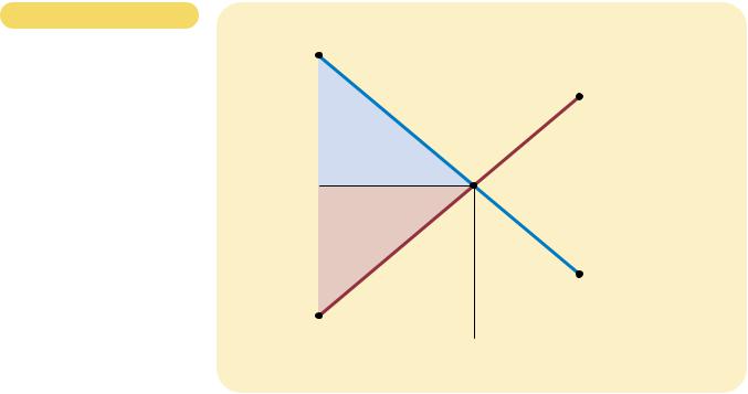
Figure 7-7 shows consumer and producer surplus when a market reaches the equilibrium of supply and demand. Recall that consumer surplus equals the area above the price and under the demand curve and producer surplus equals the area below the price and above the supply curve. Thus, the total area between the supply and demand curves up to the point of equilibrium represents the total surplus from this market.

Is this equilibrium allocation of resources efficient? Does it maximize total surplus? To answer these questions, keep in mind that when a market is in equilibrium, the price determines which buyers and sellers participate in the market. Those buyers who value the good more than the price (represented by the segment AE on the demand curve) choose to buy the good; those buyers who value it less than the price (represented by the segment EB) do not. Similarly, those sellers whose costs are less than the price (represented by the segment CE on the supply curve) choose to produce and sell the good; those sellers whose costs are greater than the price (represented by the segment ED) do not.

These observations lead to two insights about market outcomes:

ef ficiency

the property of a resource allocation of maximizing the total surplus received by all members of society

equity

the fairness of the distribution of well-being among the members of society

154	PART THREE SUPPLY AND DEMAND II: MARKETS AND WELFARE

Figur e 7-7

CONSUMER AND PRODUCER

SURPLUS IN THE MARKET

EQUILIBRIUM. Total surplus— the sum of consumer and producer surplus—is the area between the supply and demand curves up to the equilibrium quantity.

Price	A
		D
		Supply
	Consumer
	surplus
Equilibrium	E
price
	Producer
	surplus
		Demand
		B
	C
0	Equilibrium	Quantity
	quantity

1.Free markets allocate the supply of goods to the buyers who value them most highly, as measured by their willingness to pay.

2.Free markets allocate the demand for goods to the sellers who can produce them at least cost.

Thus, given the quantity produced and sold in a market equilibrium, the social planner cannot increase economic well-being by changing the allocation of consumption among buyers or the allocation of production among sellers.

But can the social planner raise total economic well-being by increasing or decreasing the quantity of the good? The answer is no, as stated in this third insight about market outcomes:

3.Free markets produce the quantity of goods that maximizes the sum of consumer and producer surplus.

To see why this is true, consider Figure 7-8. Recall that the demand curve reflects the value to buyers and that the supply curve reflects the cost to sellers. At quantities below the equilibrium level, the value to buyers exceeds the cost to sellers. In this region, increasing the quantity raises total surplus, and it continues to do so until the quantity reaches the equilibrium level. Beyond the equilibrium quantity, however, the value to buyers is less than the cost to sellers. Producing more than the equilibrium quantity would, therefore, lower total surplus.

These three insights about market outcomes tell us that the equilibrium of supply and demand maximizes the sum of consumer and producer surplus. In other words, the equilibrium outcome is an efficient allocation of resources. The job of the benevolent social planner is, therefore, very easy: He can leave the market

CHAPTER 7 CONSUMERS, PRODUCERS, AND THE EFFICIENCY OF MARKETS

155

Price			Supply
	Value	Cost
	to
		to
	buyers
		sellers
	Cost	Value
	to	to
	sellers	buyers	Demand
0	Equilibrium		Quantity
	quantity

Value to buyers is greater		Value to buyers is less
than cost to sellers.		than cost to sellers.

Figur e 7-8

THE EFFICIENCY OF THE

EQUILIBRIUM QUANTITY. At

quantities less than the equilibrium quantity, the value to buyers exceeds the cost to sellers. At quantities greater than the equilibrium quantity, the cost to sellers exceeds the value to buyers. Therefore, the market equilibrium maximizes the sum of producer and consumer surplus.

outcome just as he finds it. This policy of leaving well enough alone goes by the French expression laissez-faire, which literally translated means “allow them to do.”

We can now better appreciate Adam Smith’s invisible hand of the marketplace, which we first discussed in Chapter 1. The benevolent social planner doesn’t need to alter the market outcome because the invisible hand has already guided buyers and sellers to an allocation of the economy’s resources that maximizes total surplus. This conclusion explains why economists often advocate free markets as the best way to organize economic activity.

QUICK QUIZ: Draw the supply and demand for turkey. In the equilibrium, show producer and consumer surplus. Explain why producing more turkey would lower total surplus.

CONCLUSION: MARKET EFFICIENCY

AND MARKET FAILURE

This chapter introduced the basic tools of welfare economics—consumer and producer surplus—and used them to evaluate the efficiency of free markets. We showed that the forces of supply and demand allocate resources efficiently. That is,