page 338

23.3.1 State Diagrams Example

• A Complex Example - In this case we have a set of traffic lights. The lights will remain green in one direction until a pedestrian cross button is pushed. They will then turn yellow for four seconds and then turn red.

	Red	L1
	Yellow
		L2
	Green
		L3
	North/South
		Walk Button - S1

*This could be done with simple if-then logic (conditional)

	Red	L4
	Yellow
		L5
	Green
		L6
	East/West
		Walk Button - S2

• First we will describe the system variables. These will vary as the system moves from state to state. Please note that some of these together can define a state (alone they are not the states).

We have eight items that are ON or OFF
L1
L2	OUTPUTS	Note that each state will lead
L3		to a different set of out-
L4		puts. The inputs are often
L5		part, or all of the transi-
L6		tions.
S1	INPUTS
S2
A simple diagram can be drawn to show sequences for the

• We can then use outputs, or controlled variables, to indicate system states (you can also think of

page 339

these as modes).

Step 1 : Define the System States and put them (roughly) in sequence

System State
	L1 L2 L3 L4 L5 L6	A binary number
		0	= light off
		1	= light on
State Table

	State Description		#		L1	L2	L3	L4	L5	L6
	Green East/West		1		1	0	0	0	0	1
	Yellow East/West		2		1	0	0	0	1	0
	Green North/South		3		0	0	1	1	0	0
Yellow North/South			4		0	1	0	1	0	0

Here the four states determine how the 6 outputs are switched on/off.

• State transitions are determined based on inputs, and how the system changes. These events cause a change between states. Care must be taken to avoid confusing them with states.

Step 2 : Define State Transition Triggers, and add them to the list of states

	Description		#		L1	L2	L3	L4	L5	L6		transition
	Green East/West		1		1	0	0	0	0	1		S1
	Yellow East/West		2		1	0	0	0	1	0
	Green North/South		3		0	0	1	1	0	0
Yellow North/South			4		0	1	0	1	0	0

• The state transition diagram allows us to visually check for continuous loops. In a simple state diagram multiple transitions may lead to alternate paths.

page 340

Step 3 : Draw the State Transition Diagram

grn. EW	pushbutton NS (i.e., 10)

delay 4sec

first scan

yel. EW

yel. NS

delay 4sec

pushbutton EW (i.e. 01)

grn. NS

• For the previous traffic light example, add a speed up signal for an emergency vehicle.

A strobe light mounted on fire trucks will cause the lights to change so that the truck doesn’t need to stop. Modify the state diagram to include this option.

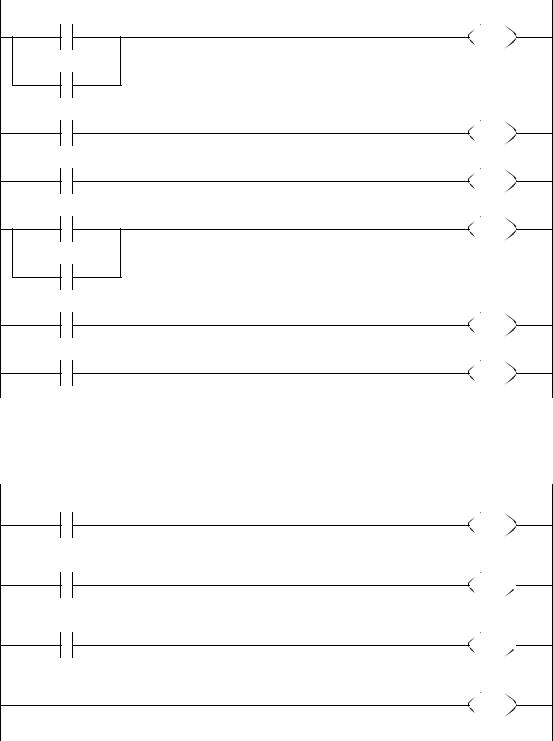
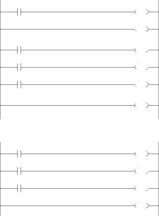
23.3.1.1 - Block Logic Conversion

• The state diagram can be implemented in ladder logic, in this case for a SLC-150. This example uses states to turn lights on or off. An initial block uses the first scan input ‘868’ to ensure the first state is state 1. Each state runs a section of ladder logic code in ‘MCR’ blocks to wait for transitions.

page 341

STATES			OUTPUTS	INPUTS
701	- state 1 - green E/W		012 - L1	101	- S1
702	- state 2	- yellow E/W	013 - L2	102	- S2
703	- state 3	- green N/S	014 - L3	868	- first scan
704	- state 4	- yellow N/S	015 - L4
			016 - L5
			112 - L6

RESET THE STATES

MCR

868

701

L

702 U

703 U

704

U MCR

page 342

TURN ON LIGHTS AS REQUIRED 701

702

704

703

703

704

702

701

FIRST STATE WAIT FOR TRANSITIONS

701

101

101

012

013

014

015

016

112

MCR

701

U

702

L

MCR

page 343

SECOND STATE WAIT FOR TRANSITIONS 702

901

901

901

THIRD STATE WAIT FOR TRANSITIONS

703

102

102

MCR

901

RTO PR 0040

702

U

703

L

901

RST

MCR

MCR

703

U

704

L

MCR

page 344

FOURTH STATE WAIT FOR TRANSITIONS
704			MCR
			902
				RTO
			PR 0040
902			704
				U
902			701
				L
902			902
				RST
			MCR

• Consider the state diagram below and implement it in ladder logic. You should anticipate what will happen if both A and C are pushed at the same time.

STA	STC
B	D
A	C
	STB

first scan

page 345

first scan

STA

B

STB

C

Note: if A and C are true at the same time then C will have priority. PRIORITIZATION is important when simultaneous branches are possible.

A C

L	STB
U	STA
U	STC
MCR
U	STA
L	STB
MCR
MCR
U	STB
L	STC
U	STB
L	STA
MCR