Rational Decision under Risk		215

able to observe what the purchaser thought the probability of each possible outcome was or the actual probability distribution. By basing choice models on experimental results, theorists have hoped to sidestep this measurement issue. In an experiment, the experimenter has the freedom to select the probabilities and outcomes and specify them exactly. This control is a substantial advantage relative to field observations, but it also creates a potential weakness. The experiments can present risky choices that do not represent the real-world choices that people face.

Many decisions are made without a clear understanding of what choices are available, what the possible outcomes of the choices are, or what the relative probability of those outcomes may be. For example, consider college freshmen considering their choice of major. Although it may be possible to determine all the possible majors available in a university, it may be difficult to know what sorts of knowledge and potential employment options would be available with each possible major. Such ambiguity about the possibilities leads nearly half of all students to change majors at least once as they discover new information that leads them in a different direction. Many students put off declaring a major until the last possible moment. Moreover, some students gain excessive credits in their search for the right major. This has led some universities (for example, the University of Wisconsin) to charge students who take too many credits, trying to encourage earlier decisions and earlier graduations. The latter portion of this chapter describes economic theories of how people deal with ambiguous choices such as these, as well as their impact on outcomes.

The ease with which people can introduce and test models of decision under risk has led to the introduction of dozens of competing models. In this chapter and the next I present the most important behavioral concepts arising from the behavioral risk literature, including only a small selection of the models that have been proposed. The interested reader who wishes to see a broader treatment of models of decision under risk is directed to the literature review compiled by Chris Starmer.

Rational Decision under Risk

Frank Knight, in his 1920s work on the importance of risk, distinguished between the terms risk and uncertainty. Knightian risk refers to a situation in which the outcome is not known with certainty but in which the decision maker knows all the possible outcomes and the probabilities associated with each (or at least has a subjective understanding of the probabilities). Gambles taken in a casino clearly fall into this category, as do most financial investments. Alternatively, Knightian uncertainty refers to situations in which either the set of possible outcomes or the probabilities associated with those outcomes are not known. Risk faced because of potential unforeseen and unknowable catastrophes may be classified as resulting in Knightian uncertainty. For example, before September 11, 2001, no one had experienced a calamitous terror attack on U.S. soil such as the attacks on New York and Washington, D.C. Having never experienced it, it would be difficult for people to know the range of possible financial implications for investors or the likelihood of any of those possible outcomes. People fearing a total collapse may be led to pull all of their money from stocks for fear of the unknown and unknowable. Knightian uncertainty is now more commonly referred to in the literature as ambiguity

	216		DECISION UNDER RISK AND UNCERTAINTY

to avoid potential confusion with the term risk. As is common, I use the terms “risk” and “uncertainty” interchangeably, referring to Knightian uncertainty as ambiguity.

Expected utility theory is the most commonly accepted rational model of decision under risk. This model supposes that people select the choice that provides the highest expected utility of wealth. Expected utility theory was first proposed by Daniel Bernoulli in 1738 in an attempt to solve the St. Petersburg paradox. Suppose you had the possibility of playing a game. If you play the game, a coin would be tossed n times, where n was the number of tosses required before the first heads was tossed. Then, you would receive $2n. If such a game were available, how much would you be willing to pay in order to play? In the early 1700s, many had thought that the expected value of the payout of the gamble might be a good model of the value of such a game, but it seems implausible that anyone would be willing to pay the expected value for this particular game. In this particular game, the expected value is given by

E x = 0.5 × 2 + 0.5 × 0.5 × 22 + 0.5 × 0.5 × 0.5 × 23 + =	0.5 i × 2i = 1 = .
i = 1	i = 1
	9 1

If someone maximized the expected payout, he would be willing to pay any finite price to play this game. Bernoulli believed that people must value money differently depending on how much they had accumulated. Thus, a dollar might not be worth as much to a billionaire as to one with only a couple hundred dollars to his name. This led Bernoulli to posit that people instead maximize their expected utility of wealth. For example, suppose the gambler’s utility function were the natural log function (which displays a diminishing slope). In this case, the expected utility would be

E U x =	0.5 i × ln 2i = ln 2	i 2i 1.39,	9 2
i = 1		i = 1

which is equal to the utility that would be obtained by gaining $4. Thus, this person would be willing to pay at most $4 to play the game.

This model is considered rational because it is based on a series of three rational axioms. A rational axiom is a rule for making rational choices that the economist generally assumes all decision makers must adhere to. Let (read “preferred to”) be a set of rational preferences. Then must satisfy the order, continuity, and independence axioms. We focus primarily on the order and independence axioms, because these are the central motivation for many behavioral models of risky choice.

The Order Axiom

Preference, , must be complete and transitive. Completeness implies that if A and B are any two gambles, then either A B (meaning A would be chosen over B), B A, or A B (meaning the gambler is indifferent between A and B). Additionally, transitivity implies that if A, B, and C are any three gambles, and A B and B C, then A C.

Rational Decision under Risk		217

The order axiom imposes the same requirements on choice under uncertainty that rationality demands for choice under certainty (see the discussion of completeness and transitivity in Chapter 1). Thus, a gambler must be able to evaluate all possible gambles and must have preferences that do not cycle. Thus, any gamble that is better than a particular gamble must also be better than all gambles that are worse than that particular gamble.

The Continuity Axiom

If A B C, then there is exactly one value r such that neither B nor the compound gamble that yields the gamble A with probability r and the gamble C with probability 1 − r are preferred; we write this as rA + 1 − rC B. Further, for any p > r, the compound gamble that yields the gamble A with probability p and the gamble C with probability 1 − p is preferred to B (we write this pA + 1 − pC B), and for any q < r, B is preferred to the compound gamble that yields the gamble A with probability q and the gamble C with probability 1 − q, or B qA + 1 − qC.

The continuity axiom requires that making small increases in the probability of a preferred gamble must increase the value of that gamble. For a full definition and discussion of the order and continuity axioms, see the Advanced Concept box at the end of the chapter. The independence axiom is described in detail later.

People who make decisions complying with the order, continuity, and independence axioms behave as if they are trying to maximize the expected utility of wealth resulting from the gamble. Thus, the utility of a probability p of obtaining $100 and 1 − p of obtaining $0 can be represented as p u100 + 1 − p u0, which is just the expected utility of the gamble. This provides the result that those who obey these three rational axioms will behave as if they are maximizing their expected utility when facing any choice involving risk.

Expected utility theory also implies that a stochastically dominant gamble is always chosen. For example, suppose you were presented a choice of

Gamble X:	Gamble Y:
0.4 probability of winning $10	0.5 probability of winning $11
0.6 probability of winning $3	0.5 probability of winning $3

In this case, Gamble Y always yields a higher probability of a larger amount of money. Let PX > k be the probability that the result of Gamble X is larger than $k. Formally, we say Gamble Y stochastically dominates Gamble X if PX > k ≤ PY > k for all values of k. Thus, a gamble that has a higher probability of a larger prize for every prize level is stochastically dominant. For example, PX > 3 = 0.4 < PY > 3 = 0.5. As well, PX > 10 = 0 < PY > 10 = 0.5. This same relation would hold no matter what value k we choose.

Any time a Gamble Y stochastically dominates X, then zPY = zUz ≥ zP X = z U z , implying that the person will always choose Y. To see this, note that

	218		DECISION UNDER RISK AND UNCERTAINTY

zPY = zUz ≥zPX = zUz is equivalent to zPY = z − PX = zUz ≥ 0, which must be the case if Y stochastically dominates X and utility is positive valued. In

this case, it seems like any reasonable decision maker would want to choose Y. In this example, Gamble Y dominates Gamble X. However, more generally it is not always possible to find a stochastically dominant gamble. For example, consider

	Gamble X′:	Gamble Y′:
	0.6 probability of winning $10	0.5 probability of winning $11
	0.2 probability of winning $3	0.3 probability of winning $3
	0.2 probability of winning $0	0.2 probability of winning $0
In this case, P X > 3 = 0.6 > P Y > 3		= 0.5, but P X > 10 = 0 < P Y > 10 =
0.5. Thus, neither gamble dominates.

EXAMPLE 9.1 Creating a Money Pump

Many have argued that people must display transitive preferences because anyone who did not have transitive preferences would be the subject of a money pump. For example, if Terry displayed preferences such that A B C A, Robin, wishing to take advantage of Terry, could offer Terry the chance to play gamble A for free. Then, once Robin has guaranteed Terry a play of gamble A, Robin could offer Terry gamble C if Terry pays Robin some small amount of money. Once Terry is endowed with C, Robin could offer to trade Terry B if Terry pays Robin some small amount of money. Robin could then offer Terry A for some small amount of money and start the process all over again. If Terry’s preferences were stable and intransitive, Robin could theoretically continue to do this until Terry was out of money. It seems unlikely that such a scheme would work in practice. Nonetheless, this might not doom the concept of intransitive preferences.

Suppose you were given a series of choices between possible gambles. Suppose you could first choose between

Gamble A:	Gamble B:
0.4 probability of winning $10	0.7 probability of winning $7.50
0.6 probability of winning $3	0.3 probability of winning $1

Graham Loomes, Chris Starmer, and Robert Sugden found that about 51 percent of participants in experiments would choose Gamble B over Gamble A. Suppose next you were asked to choose between

Gamble C:	Gamble D:
1.0 probability of winning $5	0.7 probability of winning $7.50
	0.3 probability of winning $1

		Rational Decision under Risk			219
Of participants in their experiment, about 88 percent chose Gamble C over
Gamble D. Finally, consider a choice between
	Gamble E:	Gamble F:
	0.4 probability of winning $10	1.0 probability of winning $5
	0.6 probability of winning $3

Of participants in the experiment, about 70 percent chose Gamble E over Gamble F. Note however, that Gamble E and Gamble A are identical, as are Gambles B and D and Gambles C and F. Nearly 30 percent of participants chose A, C, and F, implying that A B C A. Several similar sets of gambles were offered to 200 participants, with 64 percent displaying some preference cycle with at least one set of gambles. Thus, a majority of people appear to be subject to intransitive preferences, a violation of the order axiom.

In fact, experiments have found systematic intransitivities in individual preferences over gambles. These intransitivities are called preference reversals. This pattern of preference reversals was first discovered by Sarah Lichtenstein and Paul Slovic, who asked participants in their experiments to perform two distinct tasks. First, participants were asked to choose among pairs of gambles. Then, after some passage of time, people were asked to bid on each gamble individually, revealing their willingness to pay for each gamble. Each gamble consisted of some simple probability of winning some specified amount of money, and the remaining probability was assigned to the chance of losing some specified amount of money. In the choice experiment, gambles were paired so that one of the gambles had the possibility of winning a larger amount of money (called the $-bet, pronounced “dollar-bet”), while the other would have a larger probability of winning a positive amount of money (called the P-bet).

Lichtenstein and Slovic found that although people tended to choose P-bets over $-bets, they would often bid higher amounts for the $-bets. This is similar to the pattern of behavior above, where Gamble A represents the $-bet and Gamble B represents the P-bet. Here the P-bet is valued at less than $5 and the $-bet is valued at more than $5. However, many people tended to take the P-bet over the $-bet. Lichtenstein and Slovic’s experiment was repeated on the floor of a Las Vegas casino, with patrons given the chance to switch gambles repeatedly without ever playing a gamble. Many actually fall into the money pump trap, though most eventually discovered their irrationality. If you go to Las Vegas, beware of experimental economists. In fact, economists’ skepticism about the potential violation of the order axiom has made this one of the most tested and confirmed phenomena in behavioral economics.

EXAMPLE 9.2 Stochastic Inferiority

It might seem surprising to find violations of stochastic dominance, but in fact it is relatively easy to find examples in economic experiments. The most famous example was given by Daniel Kahneman and Amos Tversky, who asked 124 people to choose between two lotteries described by the percentage of marbles of different colors in a box

	220		DECISION UNDER RISK AND UNCERTAINTY

and the amount of money that would result from a particular color marble being drawn at random.

Gamble A:			Gamble B:
Marbles	Money		Marbles	Money
90% white	$0		90% white	$0
6% red	win $45	7% red		win $45
1% green	win $30	1% green		lose $10
3% yellow	lose $15	2% yellow		lose $15

Participants were told they would be chosen at random, with those selected facing real money outcomes from their choices. Clearly Gamble B stochastically dominates Gamble A. In B there is only a 2 percent chance of losing $15, with the remaining 1 percent chance now allocated to the possibility of losing $10. Gamble B has an additional 1 percent chance of winning $45, reallocated from the 1 percent chance of winning $30 in A. Nearly 60 percent of those participating chose gamble A, however. People were attracted to the choice with fewer negative outcomes and more positive outcomes, even though the choice with fewer negative outcomes was not as favorable.

Presenting the gambles in a way that makes the dominance clear leads to a much higher percentage identifying the dominant option. For example, when asked to choose between

Gamble C:			Gamble D:
Marbles	Money		Marbles	Money
90% white	$0		90% white	$0
6% red	win $45	6% red		win $45
1% green	win $30	1% green		win $45
1% blue	lose $15	1% blue		lose $10
2% yellow	lose $15	2% yellow		lose $15

all respondents chose Gamble D. When gambles are presented in a convoluted fashion, people appear to resort to heuristics and rules of thumb to make their choices. We refer to the clarity of presentation as the transparency. When choices are presented in a transparent way, behavioral anomalies are often minimized. Michael Birnbaum and Juan Navarrete have found violations of dominance owing to lack of transparency to be a common phenomenon in economics experiments.

Modeling Intransitive Preferences: Regret

and Similarity

Three primary explanations have been given for why we observe the violations of the order axiom. The first is based on the notion that preference reversals are simply evidence that people use different processes to perform the differing tasks (in this case choosing

Modeling Intransitive Preferences: Regret and Similarity			221
versus valuing). Thus, the probabilities and values enter into the decision process dif-
ferently depending on which task the person is asked to perform. For example, when asked
to formulate their willingness to pay, people may be drawn to anchor on the amount of
money that can be won, and then adjust downward for the uncertainty. This likely leads to
higher willingness to pay measures for bets involving larger amounts of potential win-
nings. Alternatively, when asked to choose between two gambles, the person might place
more emphasis on the probabilities involved, opting for safer bets. Although this is
probably the majority view of economists, Loomes, Starmer, and Sugden’s experiment
was designed primarily to combat the notion that response mode is the only source of
preference reversals. In their experiment described in Example 9.1, they were careful not
to ask for the person to formulate a willingness to pay but rather to ask which of two
gambles the person preferred in each case, including several degenerate gambles.
Graham Loomes and Robert Sugden proposed regret theory as a procedurally
rational explanation for why preference reversals occur. Regret theory supposes that
someone’s preference for a gamble depends upon the other possible options that may be
chosen. Thus, we could not represent someone’s valuation of a single gamble as we do
when employing expected utility. Rather, we would need to know what options he is
trading off. More specifically, regret theory supposes that a person has a utility function
given by U x, y , where x represents the money or object the person obtains and y
represents the outcome of the option forgone. We call this the regret theory utility
function. Whereas increasing x leads to higher utility, increasing y decreases utility as
people feel more and more disappointed that they did not choose the forgone gamble. For
example, if one received $5 when the alternative would have yielded $1, one feels better
than if the alternative yielded $20. Regret theory supposes that people maximize the
expectation of the regret theory utility function.
The regret theory utility function displays two important additional properties. First,
for all outcomes x, y, U x, y = − U y, x	and U x, x = 0. A regret theory utility
function meeting these conditions is called skew symmetric. The skew-symmetric
property implies that the positive utility experienced from an outcome of $10 when the
alternative was $5 is exactly the additive inverse of the negative utility experienced
when the person received $5 and could have received $10. Thus, some symmetry of joy
or disappointment is required. Second, for	any outcomes x > y > z, it must be that

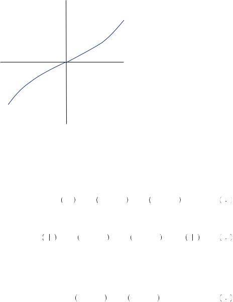
Uz, x < Uy, x + Uz, y. This property is called regret aversion. This implies that the regret felt when one obtains the lowest prize when the highest was the alternative is greater than the loss felt when obtaining the middle when the highest was the alternative plus the regret felt when obtaining the lowest when the middle was available. In other words, one would prefer two small disappointments to one large disappointment. An example of the regret utility function is displayed in Figure 9.1. You will quickly notice that this function is very similar to that of the prospect theory value function except that it is concave to the left of x = y and convex to the right. Instead of a reference point, we now have an alternative outcome at the origin. Regret aversion implies that the slope of the utility function must be increasing as the difference between x and y increases. Holding y constant, this is displayed in the figure by an increasing slope as x increases above y and an increasing slope as x decreases below y.

Suppose Dominique could bet on one of two football teams that were playing each other: team A and team B. If Dominique bets on team A and team A wins, Dominique

	222		DECISION UNDER RISK AND UNCERTAINTY

x = y

u (x, y)

x

FIGURE 9.1

The Regret Theory Utility Function Holding y Constant

receives $100. If Dominique bets on team A and team B wins, Dominique loses $100. Alternatively, suppose that if Dominique bets on team B and team B wins, Dominique will receive $50, but if team B loses, Dominique will lose $50. Finally suppose that the probability that team A wins is 0.3. Then the expected regret utility of choosing team A given B is available would be

EU A B = 0.3U 100, − 50 + 0.7U − 100, 50

9 3

and of choosing team B when A is available would be

EU B A = 0.3U − 50, 100 + 0.7U 50, − 100 = − EU A B

9 4

This last equality is a result of the skew-symmetric property. It must always be the case that the expected regret utility of one choice is exactly the negative of the expected regret utility of the other. Thus, we need only examine whether the expected regret utility of any one choice is positive to determine which will be chosen. Thus, bet A would be chosen if

0.3U 100, − 50 + 0.7U − 100, 50 > 0.

9 5

Consider the choices presented in Example 9.1, only now let us rewrite Gambles A, B, and C as in Table 9.1, which represents the gambles presented in the first example, only in terms of alternative states of the world with stable probabilities. In this case, a state of the world consists of a specified outcome for each of the possible gamble choices. This is truly how Loomes, Starmer, and Sugden presented the gambles in the experiments described in Example 9.1. Thus, the outcomes of the gambles were correlated (which does not alter the calculation of expected utility).

		Modeling Intransitive Preferences: Regret and Similarity						223
	Table 9.1 Three Gambles (see Example 1)
				State
		1		2	3
	Probability	0.4		0.3	0.3
	Gamble A	10.00		3.00	3.00
	Gamble B	7.50		7.50	1.00
	Gamble C	5.00		5.00	5.00

Given a choice of A and B, B will be chosen if
EU B A = 0.4U 7.5, 10 + 0.3U 7.5, 3 + 0.3U 1, 3	> 0.	9 6
Further, given a choice of B and C, C will be chosen if
EU C B = 0.4U 5, 7.5 + 0.3U 5, 7.5 + 0.3U 5, 1	> 0.	9 7
Finally, given a choice of A and C, A will be chosen if
EU A C = 0.4U 10, 5 + 0.3U 3, 5 + 0.3U 3, 5 > 0.		9 8

Regret aversion can explain this behavior if equations 9.8, 9.9, and 9.10 can all hold simultaneously. For now, let us assume equations 9.8 and 9.9 hold, meaning that A B, and C B. These two are not, by themselves, a violation of order and could be reconciled with expected utility theory. However, given A B, and C B, expected utility theory could not allow A C. Equation 9.9 implies that A C under regret theory. Let us examine if equation 9.10 could hold given that equations 9.8 and 9.9 both hold. The possible outcomes of the three gambles in state 1 are 10 > 7.5 > 5. The property regret aversion tells us that U5, 10 < U7.5, 10 + U5, 7.5. Multiplying by −1 and noting that skew symmetry implies U10, 5 = − U5, 10, we find

U 10, 5 > − U 5, 7.5 − U 7.5, 10 .

9 9

The possible outcomes in state 2 are 7.5 > 5 > 3. Regret aversion implies U3, 7.5 < U5, 7.5 + U3, 5. Subtracting U5, 7.5 from both sides and noting that skew symmetry implies U3, 7.5 = − U7.5, 3, yields

U 3, 5 > − U 7.5, 3 − U 5, 7.5 .

9 10

The possible outcomes in state 3 are 5 > 3 > 1, with regret aversion implying U1, 5 <

U 3, 5	+ U 1, 3 . Subtracting U 1, 3 from both sides and noting that skew symmetry
implies	U 5, 1 = U 1, 5 yields
	U 3, 5 > − U 1, 3 − U 5, 1 .	9 11

	224		DECISION UNDER RISK AND UNCERTAINTY

The left side of inequalities 9.11, 9.12, and 9.13 are all the possible outcomes of choosing A when C was available (see equation 9.10). Thus, the restrictions implied by regret aversion and skew symmetry are that EUAC > − EUBA − EUCB. Because the right side of this inequality is negative (by equations 9.8 and 9.9), any value of EUAC that is positive will satisfy both regret theory and equation 9.10. Thus, the theory permits the type of preference cycling implied by equations 9.8 to 9.10.

But not all types of preference cycling are permitted by regret theory. If A is chosen over B,

EU B A = 0.4U 7.5, 10 + 0.3U 7.5, 3 + 0.3U 1, 3 < 0.

9 12

And if B is chosen over C

EU C B = 0.4U 5, 7.5 + 0.3U 5, 7.5 + 0.3U 5, 1 < 0.

9 13

Now, equations 9.11, 9.12, and 9.13 imply that EUAC > − EUBA − EUCB > 0, thus A must be chosen over C in this case. Thus, although A C B A is possible, A B C A is not. In fact, experiments have found a far greater percentage of those who violate the order axiom are of the nature predicted by regret aversion than of the nature that are excluded by regret aversion. In other words, if people evaluate individual gambles by considering the regret they will feel if unchosen options turn out to be best, then we should expect some sorts of intransitivity. In particular, the person will always cycle toward gambles that provide the lowest average regret. In this case, each gamble dominates at least one other choice in two of three states of the world, leading each to be preferred to one other option. Similarly, the person might violate stochastic dominance if the best outcomes of the inferior gamble are always paired with the worst outcomes of the dominant gamble (see the second thought question).

Notably, we have shown this result with distributions for each option that are statistically dependent. In other words, this result occurs because of the specific outcomes that occur in the same state. For a given set of preferences, the possibility of preference cycling might depend on whether the gambles were independent (so that the outcome of one does not provide us any information about the outcome of another). If the gambles are independent then these preference cycles would not occur. Regret theory still predicts preference cycling under independent gambling alternatives. It also predicts that some people will display preference cycling for dependent gambles but not for gambles with identical probabilities for each outcome that are statistically independent. Thus, some might choose A C B A when the gambles are presented as in Table 9.1 but not when presented as in Example 9.1.

Ariel Rubinstein proposed an alternative procedurally rational decision mechanism that can account for this particular pattern of preference cycling based on similarity. Rubinstein proposes a three-stage process for choosing between two gambles. First, the gambler inspects the gambles, determining if one stochastically dominates the other. If one is stochastically dominant, that gamble is chosen. If neither of the gambles is stochastically dominant, then the gambler compares the probabilities and the outcomes of the gambles. If the probabilities are similar, then one would make the decision based upon the outcomes. If the outcomes are similar, one would make the decision based upon

Modeling Intransitive Preferences: Regret and Similarity		225

the probabilities. If neither is similar, then the gambler would base the decision on some other mechanism. As an example, consider a pair of gambles

Gamble X:	Gamble Y:
px probability of winning $x	py probability of winning $y
1 − px probability of winning $0	1 − py probability of winning $0

Write r q if r and q are close enough that the gambler perceives them to be similar.

Rubinstein’s decision steps may be outlined as:

Step 1: If both x > y and px > py then Gamble X is chosen. If both y > x and py > px then Gamble Y is chosen. If neither holds, then move to Step 2.

Step 2: If py px but x y then choose the gamble with the greater payout. If x y but px py then choose the gamble with the larger probability of payout. If neither condition holds, then move to Step 3 (which is not specified).

Jonathan Leland modified Rubinstein’s mechanism to consider more-complicated gambles. In essence, he proposes that Step 1 consider the expected utility of the gambles. If the expected utility of both gambles is similar (in other words, there is no clearly dominant gamble), then probabilities and outcomes would be compared to decide. Although Rubinstein’s original formulation excludes the possibility that a gambler would choose a stochastically dominated gamble, this generalization allows it in the case that both gambles generate similar expected utility.

Consider again the choices outlined in Example 9.1. When comparing Gamble A to Gamble B, neither stochastically dominates the other. In comparing the gambles, $7.50 may be considered similar to $10, and $3 may be considered similar to $1. However, 0.7 (attached to $7.50) is much larger than 0.4 (attached to $10). Thus the gambler may be led to choose B. In comparing C and D, again neither stochastically dominates. If $5 and $7.50 are considered similar, then the gambler would clearly choose C, with a probability 1 of obtaining the payout. In comparing E and F, $3 may be similar to $5, and $10 is much larger. Thus, the gambler may be led to choose E, displaying the observed behavioral pattern. This explanation of preference cycling, however, does not appeal to the dependence or independence of the gambles involved. Thus, similarity predicts that preference reversals should occur about as often in independent and dependent gambles. In fact, Leland finds that preference reversals are as likely to occur with independent gambles as they are to occur with dependent gambles.

EXAMPLE 9.3 Lotteries, Litigation, and Regret

Those who run publicly sanctioned lotteries have long searched for innovative ways to induce potential customers to buy. This has led to a wide variety of scratch-off games and various other lottery mechanisms. Lottery players in the Netherlands are offered two variants of a lottery for their gaming pleasure. The first is a standard lottery in which one buys a ticket and selects a number, and if the number is drawn one wins. The second