330		NAÏVE PROCRASTINATION

Although the impact of consumption on any one day probably has a very minimal impact on long-term weight, let us suppose that equation 12.51 holds. Moreover, because every period after period 2 can be described by the same discount factors and utility functions, if equation 12.51 holds, then every period thereafter people plan to eat healthy food.

Alternatively, consider period 1. If equation 12.51 holds, then in this period people choose to eat healthy food if

u x	, w1 + β		t = 3	δt − 2u x , wt xi = x , i = 1
h					h		h		12 53
> u x		, w1 + β			δt − 2u x	, wt x1	= x	, xi = x
			t = 3						, i = 2
	l				l		l	h

or if the difference in instantaneous utility of consumption is less than the discounted utility of the difference in weight. However, now the discount includes the factor β

t = 3

δt − 2u x , w

t

x

1

= x , x

= x

, i = 2

β

l

l

i

h

> ul − uh.

12 54

−

t = 3 δt − 2u xh, wt xi = xh, i = 1

The right-hand side of equation 12.54 must be identical to the right-hand side of equation 12.52. The left-hand side of equation 12.54 is equal to the left-hand side of equation 12.52 multiplied by β. If β is small enough, then the person will decide to indulge today and go on a diet tomorrow. The problem arises when tomorrow arrives. When tomorrow is finally here, then the β discount is now applied to period 3 and not to period 2. Thus, the person again decides to indulge but plans to go on a diet in period 3. A quasi-hyperbolic discounter will continue to plan to go on a diet tomorrow for the rest of eternity but never actually diet and never actually lose weight.

The Common Difference Effect

Decision makers are said to display the common difference effect if they violate the stationarity property. Recall that the stationarity property requires that if you choose x at time t over x′ at time t′, then you must also prefer x at time t+k to x′ at time t′ + k for all possible k. To find a violation of stationarity, we must be able to find a k such that decision makers reverse their preference despite the common difference in the passage of time when x and x′ are offered.

Thaler’s example of choosing between one apple today or two apples a day later is the classic example of violating stationarity. When offered one apple today or two tomorrow, many choose one today—a day is too long to wait to receive only one additional apple. However, if we ask the same question about one apple a year from now or two apples one year and one day from now, the preference often reverses. After waiting a year, a day doesn’t seem like very long to wait to double consumption. Hyperbolic (or quasi-hyperbolic) discounting provides one explanation for why decision makers might display the common difference effect. The discount applied to the period 1 delay is different for different starting times. Thus, for the difference between today and tomorrow it may be β, but for the difference between one year from now and one year and one day from now it may be δ > β. In fact, this would always lead one to be more patient in choices regarding distant future consumption but impulsive when considering

The Absolute Magnitude Effect		331

near-term consumption. Thus, people often pass up far superior outcomes that require a small delay in the near term, potentially leading to regret.

One alternative procedural explanation is that people compare relative time intervals and make decisions based upon approximations and similarity. For example, a one-day wait might loom large when compared to immediate consumption. One looks large when compared to zero. However, one year might seem to be almost identical to waiting one year and one day. Some forms of the common difference effect may be the result of rounding errors, or comparison effects, used to reduce the problem into simpler terms.

The Absolute Magnitude Effect

People also appear to apply different discounts depending on the absolute size of money rewards involved. For example, recall the experiments of Benzion, Rapoport, and Yagil displayed in Table 12.2. Note that when the participants were asked about $5,000 outcomes, discount factors hovered between 0.85 and 0.90 and did not alter much over time. Alternatively, when the amounts were smaller, discount factors in the first six months were between 0.62 and 0.71, eventually rising to the 0.85 range for longer periods of time. It has generally been observed that when larger amounts are involved, people discount much less than for smaller amounts. These results are very similar to those found by Richard Thaler, displayed in Table 12.3. Participants expressed that they were on average indifferent between receiving $15 now or $60 in one year—four times as much. Alternatively, they were indifferent to receiving $3,000 now or $4,000 in one year—only 1.25 times as much. This is a substantial difference.

Some have suggested that the difference in discount factors by outcome size is due to the fact that researchers have not measured utility but only monetary value of outcomes. If people display diminishing marginal utility of money, then the discount factor calculated from questions about indifference between bundles of money in different time periods should not produce the discount factor used by the decision maker. Consider if one is indifferent between $15 now or $60 in 1 year. We would then calculate an empirical discount factor, the factor calculated in monetary terms, to satisfy 15 = δ60, or δ = 0.25. Alternatively, the decision maker calculates by employing her utility function, according to

	U 15	= δU 60 .	12 55
Table 12.3 Estimated Discount Factors for Different Amounts
and Lengths of Time
		Time Delay
Amount	3 Months	1 Year	3 Years
$15	0.265	0.418	0.613
$250	0.578	0.746	0.813
$3,000	0.617	0.775	0.813

Source: Thaler, R.H. “Some Empirical Evidence on Dynamic Inconsistency.” Economics Letters 8(1981): 201–207.

	332		NAÏVE PROCRASTINATION

FIGURE 12.8

Approximating a

Utility Function

U			Û3,000(x)
		Û15(x)	U(x)
15	60	3,000	4,000 x

Let’s approximate the utility	function using a linear form, U15 x = U 15 +
U′ 15 × x − 15 ,4 where U′ 15	is just the marginal utility (or slope of the utility

function) if $15 is received. Then using this approximation we can rewrite equation 12.55 as

U 15 δ15 U 15 + 45U′ 15 .

12 56

Figure 12.8 displays such an approximation. The function U15 has the identical slope at the point x = 15 and represents the tangent line at that point. So long as we evaluate U15 close to the point where x = 15, this should provide a reasonable approximation to the value Ux. Rearranging equation 12.56, we find

	δ15		U 15		.	12	57
		U 15	+ 45U′	15
Table	12.3 suggests that δ15		0.418,	implying		that U 15 U 15	+
45U′ 15	0.418. Suppose U 15 = 15. Then,			U′ 15		0.4641, giving us	an

approximation of the marginal utility of wealth at x = 15. Alternatively, if one is indifferent between $3,000 now or $4,000 in one year, then

U 3000 = δU 4000 .	12 58
Now let us consider a similar approximation U3000 x = U 3000	+ U′ 3000 ×

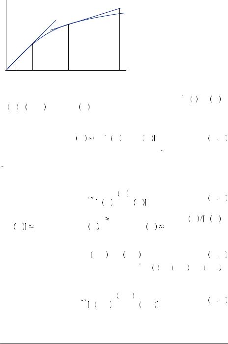
x − 3000, also displayed in Figure 12.8 (though clearly not to scale). Substituting into

equation 12.58 and rearranging as before, we find
	U 3000
δ3000		.	12 59
	U 3000 + 1000U′ 3000

We want to determine if it is possible that we would observe the person being indifferent between $3,000 now or $4,000 in one year if the discount factor were stable over both this

4 This is commonly referred to as a Taylor series approximation around the point x = 15. You might recognize this from introductory calculus coursework.

						The Absolute Magnitude Effect				333
decision and the one involving $15 now versus $60 one year from now. Suppose
that	δ3000 = δ15 = 0.418.		Then,	U 3000	U 3000	+ 1000U′ 3000	0.418, or
U′	3000	0.00139 × U 3000 . Moreover,			because	of diminishing marginal		utility,
U 3000		must fall below U15 3000 , as depicted in Figure 12.8. Thus,
U 3000 <U 15 +U′ 15 × 3000 −15					15 +0.4641 ×2985 =1400 3385.			12 60
Thus,
		U′	3000	0 00139 × U 3000		< 1 949,		12 61

which would clearly be satisfied by any utility function displaying diminishing marginal utility given U′15 0.1935. In other words, indifference between $3,000 now and $4,000 a year from now may be due to diminishing marginal utility (the extra $1,000 is not as valuable to the recipient) instead of an inflated discount factor. Thus, although we have some evidence that larger amounts of money are discounted less heavily, it is unclear whether this result represents true underlying preferences or if it just the result of a shortcoming in our methods used to elicit discount factors.

The absolute magnitude effect implies that discounting is much closer to exponential with regard to larger amounts. This means that people are much less likely to display time-inconsistent preferences for large transactions than for small transactions. Similar experiments have been conducted by several different researchers, some using real and substantial money rewards.

EXAMPLE 12.4 Gains, Losses, and Addiction

Just as people appear to discount large and small rewards differently, they also appear to discount gains and losses differently. For example, Benzion, Rapoport, and Yagil also asked the 204 participants in their study about their preferences between being forced to pay a debt of money after various waiting periods. Participants were told they owed a debt of some amount of money (e.g., $200), which was due immediately. Unfortunately they didn’t have the means to pay it. Instead, they are offered the option to make a larger payment at some future date (e.g., in six months). Participants were asked how much the payment would need to be in order to be indifferent between paying the $200 now or the higher amount later. As in the experiments over the gain domain, the amounts of money and the length of time were varied.

Table 12.4 displays the estimated discount factors for each of the various scenarios similar to the scenario just described, assuming a money metric utility function. In every case, the participant discounts future utility less when facing a loss than when facing a gain. When facing the prospect of a loss, suddenly future utility is more valuable. Again, we can see that larger amounts lead to larger discount factors, less discounting, and discounting that appears to be closer to the exponential model. In this case, however, it is more of a puzzle. The data suggest that people are indifferent between gaining

	334		NAÏVE PROCRASTINATION
			Table 12.4 Estimated Discount Factors for Different Amounts
			and Lengths of Time
							Time Delay
			Amount	6 Months		1 Year	2 Years	4 Years
			Losses
			−$40	0.749		0.820	0.838	0.876
			−$200	0.794		0.857	0.864	0.887
			−$1,000	0.822		0.866	0.868	0.892
			−$5,000	0.867		0.905	0.919	0.930
			Gains
			$40	0.626		0.769	0.792	0.834
			$200	0.700		0.797	0.819	0.850
			$1,000	0.710		0.817	0.875	0.842
			$5,000	0.845		0.855	0.865	0.907

Source: Benzion, U., A. Rapoport, and J. Yagil. “Discount Rates Inferred from Decisions: An Experimental Study.”

Management Science 35(1989): 270–284.

$40 now or $52 in one year. Using analysis similar to that in the previous section, this implies

U 40 = δU 52 .

12 62

Substituting U40x into (12.62) leads us to

U 40	12 63
δ40 U 40 + 12U′ 40 .

Table 12.4 suggests that δ40 0.769, implying that U40U40 + 12U′40 0.769. Suppose U40 = 40. Then, U′40 1.00. Table 12.3 also implies that people are indifferent to paying $40 now, or $49 one year from now. If one is indifferent between paying $40 now or $49 in one year, then

U − 40 = δU − 49 .

12 64

Substituting U − 40x into (12.64) obtains

δ − 40	12 65
U − 40 − 9U′ − 40 .

We are again interested in determining if it is possible that the same discount factor could explain being indifferent between gaining $40 now or $52 in the future also explains being indifferent between losing $40 now or losing $49 in the future. Thus, suppose that δ − 40 = δ40 = 0.769. Then, U− 40U− 40− 9U′− 40 0.769, or U′− 40 − 0.03338 × U− 40. Diminishing marginal utility tells us that U− 40 < U40− 40, or

U − 40 < U 40 + U′ 40 × − 40 − 40 40 − 1.00 × 80 = − 40,

12 66

	The Absolute Magnitude Effect			335
which implies that
U′ − 40	− 0.03338 × U − 40 < 1.3351.	12 67

Note that 1.3351 > 1.00 = U′(40). Thus, this difference in discount factors may be due to diminishing marginal utility, or due to some difference in discounting between gains and losses that will occur in the future.

The difference in discounting between gains and losses, called gain–loss asymmetry, has been observed in several settings. For example, Amy Odum, Gregory Madden, and Warren Bickel conducted several experiments asking people about either delaying treatment of an existing disease or delaying the onset of symptoms of a disease. Specifically, participants in their study are asked to consider the following hypothetical scenario:

For the last 2 years, you have been ill because at some time in the past you had unprotected sex with someone you found very attractive, but whom you did not know. Thus, for the past 2 years you have felt tired and sometimes light-headed. Food has not tasted good. You have not found sex as desirable or enjoyable as you used to. For the past 2 years, you have come down with a lot of colds and other ailments, some of which have required hospitalization. You have lost a lot of weight and are getting increasingly thin. Some friends do not come to see you anymore because of your disorder and those who do feel uncomfortable being with you. Imagine that without treatment you will feel this way for the rest of your life and that you will not die during any of the time periods described here.5

Participants were then asked about their indifference between two treatments, one that would eliminate all symptoms immediately but last only for a limited time, or an alternative treatment that would eliminate all symptoms after some delay and last a longer period of time. Similar questions were asked regarding a different scenario in which a healthy person is told that there is a 100% chance they will begin to show symptoms of the same disease owing to a past experience with unprotected sex. They are then asked about treatments that will delay the symptoms for various lengths of time and that will be effective for various lengths of time. On average, people were willing to delay losses (in this case symptoms) more than gains (eliminating symptoms). People considering treatment for an existing disease were indifferent between 10 years of health beginning one year from now or 8.85 years of health now. When considering treatment for a newly acquired disease, 10 years of health delayed one year was equivalent to 8.25 years of health beginning immediately. Though similar to the effect found in the case of money outcomes, this is not a large difference.

The researchers conducted the same experiments on people who regularly smoke cigarettes, and they found a much wider disparity (7.75 years and 5 years, respectively). Interestingly, there is a substantial amount of research that finds greater discounting among those addicted to various substances, including cigarettes. This and other research seems to suggest a link between addiction and the onset of hyperbolic discounting. Much like the model of addiction in the previous chapter on projection bias, hyperbolic

5 Odum, A.L., G.J. Madden, and W.K. Bickel. “Discounting of Delayed Health Gains and Losses by Current, Neverand Ex-Smokers of Cigarettes.” Nicotine & Tobacco Research 4, Issue 3 (2002): 295–303, by permission of Oxford University Press.

	336		NAÏVE PROCRASTINATION

discounting can offer an explanation for addictive behaviors through time-inconsistent preferences. Essentially, people might consider the benefit of the first cigarette to be high enough to overcome the negative utility derived from next period’s stronger need for the substance. Moreover, smokers might believe that it will just be this once, because in the future they will discount in a manner that is closer to the exponential model. In that case, smokers don’t think the cigarette will be worthwhile tomorrow, and they intend to quit. But as with all the models in this chapter, the planned actions do not come to pass.

Discounting with a Prospect-Theory

Value Function

One explanation for gain–loss asymmetry may be that people do not display diminishing marginal utility of money over losses. George Loewenstein and Drazen Prelec propose that both gain–loss asymmetry and absolute magnitude effects may be reconciled by pairing the hyperbolic discount function with a prospect-theory value function displaying loss aversion in place of the standard utility function. Thus, people solve

max c1, c2, V c1, c2,	=	T	1 + αt −	β	12 68
		i = 1		α v ci k
where
v c k	ug c − k	if	c ≥ k		12 69
	ul c − k	if	c < k

as defined in previous chapters, where k is a reference point such that any level of consumption greater than k is considered a gain, and any amount less than k is considered a loss. It is common to suppress the reference point and write vz = vx − k0. As defined in prior chapters, ug is a concave function displaying diminishing marginal utility of gains, and ul is a convex function representing diminishing marginal pain from losses. Moreover, the slope of ul near the reference point is much steeper than the slope of ug near the reference point, thus yielding the familiar shape in Figure 12.5. The hyperbolic discount factor is used to explain the common difference effect, as in previous examples. But note that the discount factor in equation 12.68 does not vary by the size of c or by whether c would be considered a gain or a loss. Rather, the asymmetry of gains and losses as well as the absolute magnitude effect are explained by the shape of the value function.

Previously, it was shown how a concave function could explain the absolute magnitude effect in the domain of gains. Alternatively, the asymmetry of gains and losses cannot be explained by the standard utility function that displays diminishing marginal utility (concavity) everywhere. Reconsider the example in the previous section. If the loss function is convex, then equations 12.66 and 12.67 need not hold, and thus no contradiction is created. Thus, it is possible that the person with a single and stable discount factor for utility realized one year from now could be indifferent between $40

Discounting with a Prospect-Theory Value Function		337

Utility value

(Losses)

–ug

ul

ug

(Gains)

Dollar value

FIGURE 12.9

The Prospect Theoretic Value Function with Intermediate Loss Aversion

now and $52 a year from now and could also be indifferent between losing $40 now and losing $49 a year from now. Allowing ul to be convex eliminates the contradiction created by discounting future losses less heavily than gains. To reconcile this model with each of the observed violations of the fully additive model, we must introduce three restrictions on the value function.

First, intermediate loss aversion requires that for any c > 0, vc < − v− c. Intermediate loss aversion requires that any loss of a particular size be experienced as a larger reduction in utility than the gain in utility that would result from a gain in consumption of the same size. This requires that the value function is steeper over the loss domain than over the gain domain. We call this intermediate loss aversion because it is a slightly weaker condition than strong loss aversion as defined in Chapter 3. Any value function that displays strong loss aversion also displays intermediate loss aversion. However, it is possible to find functions that are intermediate-loss averse but not strongloss averse. Figure 12.9 displays a value function satisfying intermediate loss aversion. The function ug is reflected around the origin, resulting in the dashed curve. It is apparent that ul is everywhere below the reflected curve.

Second, the asymmetric elasticity condition requires that the utility of losses is more elastic than utility of gains. Let z2 > z1 > 0 be amounts of money. Then we can express this requirement in terms of arc elasticities

ε − z1, − z2

= −

z1 + z2

v − z1

− v − z2

>

z1 + z2

v z2

− v z1

= ε z2, z1

z2 − z1

v − z1

+ v − z2

z2 − z1

v z1

+ v z2

12 70

or for any z > 0 in terms of exact elasticities as

ε − z = −

zv′ − z

>

zv′ z

= ε z ,

12 71

v − z

v z

where ɛ is the elasticity of the value of function with respect to outcomes.

	338		NAÏVE PROCRASTINATION

This is very similar to the requirement of strong loss aversion. When coupled with intermediate loss aversion, this actually creates a condition that is more restrictive than strong loss aversion. The elasticity condition requires that the loss curve be more convex than the gain curve is concave. In Figure 12.9 this can be seen as the loss curve bends toward horizontal much more quickly as you move along the loss axis than does the reflection of the gain curve.

Finally, we must require the value function to be subproportional. Subproportionality requires that the value function increases in elasticity as the absolute value of consumption increases. Let z2 > z1 > 0, and let 0 < < z1 represent amounts of money. Then we can express this requirement in terms of arc elasticities as

ε z2, z2 + =

2z2 + v z2 + − v z2

> 2z1 + v z1 + − v z1

12 72

v z2 + + v z2

v z1 + + v z1

= ε z1,

z1 +

and

ε − z2, − z2

+ =

− 2z2 + v − z2 + − v − z2

v

− z2 +

+ v − z2

> − 2z1 + v − z1 + − v − z1

12 73

v − z1 +

+ v − z1

= ε − z1,

− z1 +

or in terms of exact elasticities as

ε z2 =

z2v′ z2

> z1v′ z1 = ε z1

12 74

v z2

v z1

and

ε − z2 = −

z2v′ − z2

> −

z1v′ − z1

= ε − z1 .

12 75

v − z2

v

− z1

This requirement imposes a minimum level of concavity (or convexity in the case of the loss domain) on the value function. Essentially, this requires that the difference in utility between relatively large outcomes must be minimal compared to the difference in utility of two relatively small outcomes of the same proportions. Another way to state

this requirement is that whenever z2 > z1 > 0, and α > 1, v z2 v αz2	< v z1 v αz1 ,
hence the name subproportionality.
If a person is indifferent between receiving z1 > 0 now or z2 > z1	at some future

specified date, then vz1 = ψtvz2, where ψt is the appropriate hyperbolic discount factor for a delay of t. If v displays intermediate loss aversion, then it will require more than z2 at the future date to compensate the person for an immediate loss of

	Discounting with a Prospect-Theory Value Function						339
z1, − v − z1 < ψ t v z2 . Thus, the person would not be willing to suffer a loss of z1 now
to obtain z2 later. Moreover, v z1 = ψ t v z2 can be rewritten as
v z2 − v z1 = 1 ψ t − 1 v z1					12 76
yielding an arc elasticity of preference
ε z1z2 =	z1 + z2 1 ψ t − 1 v z1		.		12 77
	z2 − z1 1 ψ t + 1 v z1
The arc elasticity over losses of z1 and z2 is given by
ε − z1, − z2 = −		z1 + z2 v − z1 − v − z2		.	12 78
		z2 − z1 v − z1 + v − z2

If the person displays asymmetry of elasticity of preference, then

	ε − z1, − z2	= −	z1 + z2	v	− z1	− v	− z2
			z2 − z1	v	− z1	+ v	− z2

which, by cancelling terms, is equivalent to

	>	z1 + z2	1 ψ t	− 1 v z1	= ε z1z2 ,
		z2 − z1	1 ψ t	+ 1 v z1
					12 79

v − z1 > ψ t v − z2 ,

12 80

meaning that the person would prefer losing z1 today to losing z2 at time t. Thus, if z3 is such that the person is indifferent between losing z1 today and losing z3 at time t it must be that z3 < z2 (or that − z3 > − z2).

This is important considering the phenomenon of gain–loss asymmetry. Gain–loss asymmetry is observed by asking people for the amounts of money needed to compensate them for a forgone gain or a loss. Then discount factors are calculated from the dollar amounts rather than from the unobserved utility value. So if you were asked the amount of money at time t necessary to make you indifferent to gaining z1 today you would respond z2. This would lead an economist to calculate an empirical discount factor assuming a money metric utility function by finding the δ satisfying z1 = δgz2, or δg = z1z2. Asking for the amount you would need to lose at time t to make you indifferent to an immediate loss of z1 would result in a response of z3 < z2. This would in turn lead to an empirical discount factor of δl = z1z3 > z1z2 = δg. Thus, the asymmetry of elasticity property implies behavior that is consistent with gain–loss asymmetry.

Finally, subproportionality is used to explain the absolute magnitude effect. Consider someone who is indifferent between obtaining z1 > 0 now or αz1 at some future date t, where α > 1. Using her stated indifference to calculate an empirical discount factor results in δ = z1αz1 = 1α. Now suppose we were to ask about the amount necessary at time t to compensate for not receiving z2 > z1 immediately. Subproportionality requires that

340

NAÏVE PROCRASTINATION

ε z2, z2 + αz2 =

z2 1 + α v αz2 − v z2

>

z1 1 + α v αz1 − v z1

= ε z1, z1 + αz1 ,

α − 1 z2 v αz2 + v z2

α − 1 z1 v αz1 + v z1

12 81

where each side of the above inequality is the corresponding arc elasticity from equation

12.71. Cancelling terms yields

v z1

>

v z2

.

12 82

v αz1

v αz2

Indifference

between

z1 now or αz1 at

time t implies v z1 = ψ t

v αz1 ,

or that

ψ t = v z1

v αz1 . Substituting into equation 12.82 implies that ψ t

> v z2

v αz2 ,

and thus v z2

< ψ t v αz2 , implying that the person would require less compensation

than αz2 at time t to compensate for the delay. Suppose instead that to be indifferent, the

person would need to receive z3 < αz2. Then the implied empirical discount factor would

be δ = z2 z3 > z2 αz2 = 1 α. Thus the person would necessarily display the absolute

magnitude effect if subproportionality is satisfied.

EXAMPLE 12.5

Now or Later

Impatience can lead us to want good things to happen sooner rather than later. At the heart of many of the questions of intertemporal choice is how much we are willing to pay to speed up consumption, or how much we are willing to accept to slow down consumption. Suppose you purchased a $100 gift certificate to your favorite restaurant today and paid the maximum amount that you would be willing to pay. How much would you need to be compensated today not to use the gift certificate for six months?

George Loewenstein asked a group of M.B.A. students at Wharton Business School this question, receiving an average response of $23.85. Let Ug, w be instantaneous utility, where g represents the value of any gift certificates and w represents the value of any wealth one has in addition. The person must be indifferent between her current state, the state in which she has purchased the gift certificate for her maximum willingness to pay, and the state in which she has purchased the gift certificate and has been compensated for not using the certificate for six months. Before purchasing the gift certificate, her utility would be given by U0, w1 + ψ6U0, w2. Let vnow be the maximum she would be willing to pay to receive a $100 gift certificate that could be used now. Then she must be indifferent between her current utility and the utility of purchasing that gift certificate for vnow , U100, w1 − vnow + ψ6U0, w2. Further, she must be indifferent between both of these values of utility and the utility obtained if she bought now and paid vnow , received an additional $23.85, and then could not use the certificate for an additional six months, U0, w1 − vnow + 23.85 + ψ6U100, w2. These indifference relationships imply

	U 0, w1 + ψ 6 U 0, w2 = U 100, w1 − vnow	+ ψ 6 U 0, w2	12 83
	= U 0, w1 − vnow +	23.85 + ψ 6 U 100, w2 .

		Discounting with a Prospect-Theory Value Function					341
Alternatively, a second set of M.B.A. students was asked to consider a scenario in
which they would purchase a $100 gift certificate in six months and pay the maximum
amount they would be willing to pay. They were then asked how much they would pay to
receive the gift certificate now. On average, they replied $10.17, about half as much as
the compensation for waiting. These students must be indifferent between their current
state, a state	in which they	pay today for a gift	certificate in six		months,
U 0, w1 − vlater	+ ψ 6 U 100, w2	, and the state in which they purchase the certificate
and then pay $10.17 extra		to use the certificate	now, U 100, w1 − vlater −
10.17 + ψ 6 U 0, w2 . These indifference relationships imply
U 0, w1 + ψ 6 U 0, w2 = U 0, w1 − vlater + ψ 6 U 100, w2					12 84
	=	U 100, w1 − vlater − 10.17 + ψ 6 U 0, w2 .
Note that the first terms in equations 12.83 and 12.84 are identical, and thus all terms
must be equal. This implies that
U 100, w1 − vnow + ψ 6 U 0, w2 = 100, w1 − vlater − 10.17 + ψ 6 U 0, w2				,	12 85
which requires that vnow = vlater + 10.17. Additionally,
U 0, w1 − vnow + 23.85 + ψ 6 U 100, w2 = U 0, w1 − vlater			+ ψ 6 U 100, w2	,	12 86

which requires that vnow = vlater + 23.85, which is of course a contradiction. In fact, the fully additive model always requires that the willingness to pay to speed up consumption should be identical to the willingness to accept to delay consumption.

This violation of the fully additive model, called delay–speedup asymmetry, is a common phenomenon that has been shown in many contexts. People are willing to pay between one fourth and one half as much to speed up consumption as they are willing to accept to slow down consumption.

The value function, given intermediate loss aversion, provides one explanation for this phenomenon. In this case, the framing of the question makes a difference. When using a value function to explain behavior, prior wealth is not incorporated into the reference point. The utility calculation before any transaction is now given by v0, 0 + ψ6v0, 0, where vg, w is the value of a change in gift certificates relative to the reference point of value g and a change in wealth relative to the reference point of w. When purchasing a $100 gift certificate to be used now at a price of vnow , the value is given by v100, − vnow + ψ6v0, 0. The person who first purchases the gift certificate for her maximum willingness to pay will satisfy

v 0, 0 + ψ 6 v 0, 0 = v 100, − vnow + ψ 6 v 0, 0 .

12 87

Then she is asked how much she would need to be compensated to put off consumption by six months. At this point, however, consumption has been incorporated in the reference point, as has the initial payment for the gift certificate. Thus, one considers having a gift certificate of $100 and initial wealth minus vnow to be the reference point, yielding v0, 0+ ψ6v0, 0. Giving up the certificate for six months is considered a loss in this period but a gain in the future, and the payment of $23.85 received in order to wait is considered a current-period gain, v− 100, 23.85 + ψ6v100, 0. Thus, indifference now implies

	342		NAÏVE PROCRASTINATION

v 0, 0 + ψ 6 v 0, 0 = v − 100, 23.85 + ψ 6 v 100, 0 .

12 88

Alternatively, paying initially for a coupon to be received in six months results in the indifference relationship

v 0, 0 + ψ 6 v 0, 0 = v 0, − vlater + ψ 6 v 100, 0 .

12 89

Then, when the person is asked how much she is willing to consume immediately, she considers the purchase price already to be part of the reference point. Again she is finding the amount of money that would make her indifferent between v0, 0 + ψ6v0, 0, her new current reference point, and a gain of a $100 certificate in this period and a loss of a $100 certificate in the future, v100, − 10.17 + ψ6v− 100, 0. Thus, indifference now implies

v 0, 0 + ψ 6 v 0, 0 = v 100, − 10.17 + ψ 6 v − 100, 0 .

12 90

Because of the framing of the question, the $23.85 in compensation to slow down consumption enters as a gain, and the $10.17 payment to speed up compensation is recorded as a loss. Intermediate loss aversion requires that vx<− v− x for any positive x. Thus, the gain of $23.85 has a smaller impact on utility than would a loss of $23.85.

Empirical evidence suggests losses are valued about twice the amount of an equivalent gain, offering one explanation for the delay–speedup asymmetry. Combining equations 12.88 and 12.90, we find

v − 100, 23.85 = v 0, − vlater ,

12 91

or losing the maximum willingness to pay for consumption later is equivalent to losing the gift certificate and gaining $23.85. Other comparisons are not possible given the different state of the gift certificate in the latter period. No violations of this model can occur when comparing the delay–speedup problem because values are evaluated through different functions. When delaying, the gift certificate is evaluated as a loss now and a gain later. When speeding up, it is evaluated as a gain now and a loss later. Thus, not only is the discount factor involved but the difference in the shape of the gain and loss functions are involved also, allowing the asymmetric behavior.

It is noteworthy that the delay–speedup asymmetry is primarily observed for monetary outcomes or other items with mundane value. When we consider events that involve significant emotions, people can behave much differently. For example, George Loewenstein at one point asked several participants for their maximum willingness to pay to receive a kiss from the movie star of their choice immediately. He then asked them their maximum willingness to pay for the event at several future dates. Similarly, participants were asked the amount they would need to be paid to receive a 120-volt shock either immediately or at several intervals in the future. The results of this experiment are displayed in Figure 12.10.

One would think of receiving a kiss from the movie star of your choice as being a positive thing. Nevertheless, people are willing to pay more to delay the kiss by up to one year. Waiting ten years, however, results in a steep discount. Alternatively, receiving an electric shock, though it wouldn’t kill you, would generally be considered an unpleasant experience, which generally means delay is preferred. Instead, participants had to be compensated much more if they were to receive the shock in the future rather