Introduction to 3D Game Programming with DirectX.9.0 - F. D. Luna

14 Part I

As an example, find the product:

4 1 1 3 AB

2 1 2 1

We verify the product is defined because the number of columns of A equals the number of rows of B. Also note that the resulting matrix is a 2 2 matrix. Using formula (4), we have:

4 1 1 3

a1

b1

a1

b2

4 1 1 2

4 1 3 1

6 13

AB

a

b a

b

0

2 1 2 1

2

2

2

2 1 1 2 2 1 3 1

5

1

As an exercise, verify for this particular example that AB

BA.

Y

A more general example:

L

b11

b12

F

a11b12 a12 b22 a13 b32

a11

a12

a13

a11b11

a12 b21 a13 b31

C

AB

a22

a23

b21

b22

a22 b21 a23 b31

a21

b

b

a21b11

a21b12 a22 b22 a23 b32

31

32

M

The Identity Matrix

A

E

T

There is a special matrix called the identity matrix. The identity matrix is a square matrix that has zeros for all elements except along the main diagonal, and the elements along the main diagonal are all ones. For example, below are 2 2, 3 3, and 4 4 identity matrices:

1	0	1 0		0	1 0 0			0
0	1	0	1	0	0 1 0			0
		0	0	1	0	0	1	0
					0	0	0	1

The identity matrix acts as a multiplicative identity:

MI = IM = M

That is, multiplying a matrix by the identity does not change the matrix. Further, multiplying with the identity matrix is a particular case when matrix multiplication is commutative. The identity matrix can be thought of as the number “1” for matrices.

1	2	2
Example: Verify that multiplying the matrix M	by the 2
0	4

identity matrix results in M.

Team-Fly®

Mathematical Prerequisites

1		2 1			0		1		2 1 0 1	2 0 1	1		2
	0	4		0	1			0	4 1 0 0			0	4
										4 0 1

Inverses

In matrix math there is not an analog to division but there is a multiplicative inverse operation. The following list summarizes the important information about inverses:

Only square matrices have inverses; therefore when we speak of matrix inverses, we assume we are dealing with a square matrix.

The inverse of an n n matrix M is an n n matrix denoted as M–1.

Not every square matrix has an inverse.

Multiplying a matrix with its inverse results in the identity matrix: MM–1 = M–1M = I. Note that matrix multiplication is commutative when multiplying a matrix with its inverse.

Matrix inverses are useful for solving for other matrices in a matrix equation. For example, consider the equation p = pR and suppose that we know p and R and wish to solve for p. The first task is to find R–1 (assuming it exists). Once R–1 is known, we can solve for p, like so:

p R 1 p RR 1 p R 1 pI

p R 1 p

15

P a r t I

Techniques for finding inverses are beyond the scope of this book, but they are described in any linear algebra textbook. In the section titled “Basic Transformations” we give the inverses for the particular matrices that we work with. In the section titled “D3DX Matrices” we learn about a D3DX function that finds the inverse of a matrix for us.

To conclude this section on inverses we present the following useful property for the inverse of a product: (AB)–1 = B–1 A–1. This property assumes both A and B are invertible and that they are both square matrices of the same dimension.

The Transpose of a Matrix

The transpose of a matrix is found by interchanging the rows and columns of the matrix. Thus, the transpose of an m n matrix is an n m matrix. We denote the transpose of a matrix M as MT.

16 Part I

Example: Find the transpose for the following two matrices:

2	1	8		a	b	c
			B
A				d e f
3	6	4		g h		i

To reiterate, the transposes are found by interchanging the rows and columns. Thus:

	2		3			a	d	g
AT	1 6				BT	b e h
		8	4			c	f	i

D3DX Matrices

When programming Direct3D applications, we typically use 4 4 matrices and 1 4 row vectors exclusively. Note that using these two sizes of matrices implies the following matrix multiplications are defined:

Vector-matrix multiplication. That is, if v is a 1 4 row vector and T is a 4 4 matrix, the product vT is defined and the result is a 1 4 row vector.

Matrix-matrix multiplication. That is, if T is a 4 4 matrix and

R is a 4 4 matrix, the products TR and RT are defined and both result in a 4 4 matrix. Note that the product TR does not necessarily equal the product RT because matrix multiplication is not commutative.

To represent 1 4 row vectors in D3DX, we typically use the D3DXVECTOR3 and D3DXVECTOR4 vector classes. Of course, D3DXVECTOR3 only has three components, not four. However, the fourth component is typically an understood one or zero (more on this in the next section).

To represent 4 4 matrices in D3DX, we use the D3DXMATRIX class, defined as follows:

typedef struct D3DXMATRIX : public D3DMATRIX

{

public: D3DXMATRIX() {};

D3DXMATRIX(CONST FLOAT*); D3DXMATRIX(CONST D3DMATRIX&);

D3DXMATRIX(FLOAT _11, FLOAT _12, FLOAT _13, FLOAT _14, FLOAT _21, FLOAT _22, FLOAT _23, FLOAT _24, FLOAT _31, FLOAT _32, FLOAT _33, FLOAT _34, FLOAT _41, FLOAT _42, FLOAT _43, FLOAT _44);

Mathematical Prerequisites

// access grants

FLOAT& operator () (UINT Row, UINT Col); FLOAT operator () (UINT Row, UINT Col) const;

//casting operators operator FLOAT* ();

operator CONST FLOAT* () const;

//assignment operators

D3DXMATRIX& operator *= (CONST D3DXMATRIX&);

D3DXMATRIX& operator += (CONST D3DXMATRIX&);

D3DXMATRIX& operator -= (CONST D3DXMATRIX&);

D3DXMATRIX& operator *= (FLOAT);

D3DXMATRIX& operator /= (FLOAT);

// unary operators

D3DXMATRIX operator + () const;

D3DXMATRIX operator - () const;

// binary operators

D3DXMATRIX operator * (CONST D3DXMATRIX&) const; D3DXMATRIX operator + (CONST D3DXMATRIX&) const; D3DXMATRIX operator - (CONST D3DXMATRIX&) const; D3DXMATRIX operator * (FLOAT) const;

D3DXMATRIX operator / (FLOAT) const;

friend D3DXMATRIX operator * (FLOAT, CONST D3DXMATRIX&);

BOOL operator == (CONST D3DXMATRIX&) const;

BOOL operator != (CONST D3DXMATRIX&) const;

} D3DXMATRIX, *LPD3DXMATRIX;

The D3DXMATRIX class inherits its data entries from the simpler D3DMATRIX structure, which is defined as:

typedef struct _D3DMATRIX { union {

struct {

float _11, _12, _13, _14; float _21, _22, _23, _24; float _31, _32, _33, _34; float _41, _42, _43, _44;

};

float m[4][4];

};

} D3DMATRIX;

Observe that the D3DXMATRIX class has a myriad of useful operators, such as testing for equality, adding and subtracting matrices, multiplying a matrix by a scalar, casting, and—most importantly—multiplying two D3DXMATRIXs together. Because matrix multiplication is so important, we give a code example of using this operator:

D3DXMATRIX A(…); // initialize A

D3DXMATRIX B(…); // initialize B

17

P a r t I

18 Part I

D3DXMATRIX C = A * B; // C = AB

Another important operator of the D3DXMATRIX class is the parenthesis operator, which allows us to conveniently access entries in the matrix. Note that when using the parenthesis operator, we index starting into the matrix starting at zero like a C-array. For example, to access entry ij = 11 of a matrix, we would write:

D3DXMATRIX M;

M(0, 0) = 5.0f; // Set entry ij = 11 to 5.0f.

The D3DX library also provides the following useful functions that set a D3DXMATRIX to the identity matrix, take the transpose of a D3DXMATRIX, and find the inverse of a D3DXMATRIX:

D3DXMATRIX *D3DXMatrixIdentity(

D3DXMATRIX *pout	// The matrix to be set to the identity.
);
D3DXMATRIX M;
D3DXMatrixIdentity( &M );	// M = identity matrix
D3DXMATRIX *D3DXMatrixTranspose(
D3DXMATRIX *pOut,	// The resulting transposed matrix.
CONST D3DXMATRIX *pM	// The matrix to take the transpose of.
);
D3DXMATRIX A(...);	// initialize A

D3DXMATRIX B;

D3DXMatrixTranspose( &B, &A ); // B = transpose(A)

D3DXMATRIX *D3DXMatrixInverse(

D3DXMATRIX *pOut,	// returns inverse of pM
FLOAT *pDeterminant,	// determinant, if required, else pass 0
CONST D3DXMATRIX *pM	// matrix to invert
);

The inverse function returns null if the matrix that we are trying to invert does not have an inverse. Also, for this book we can ignore the second parameter and set it to 0 every time.

D3DXMATRIX A(...);	// initialize A
D3DXMATRIX B;
D3DXMatrixInverse( &B, 0, &A );	// B = inverse(A)

Basic Transformations

When programming using Direct3D, we use 4 4 matrices to represent transformations. The idea is this: We set the entries of a 4 4 matrix X to describe a specific transformation. Then we place the coordinates of a point or the components of a vector into the columns of a 1 4 row

Mathematical Prerequisites

vector v. The product vX results in a new transformed vector v . For example, if X represented a 10-unit translation on the x-axis and v = [2, 6, –3, 1], the product vX = v = [12, 6, –3, 1].

A few things need to be clarified. We use 4 4 matrices because that particular size can represent all the transformations that we need. A 3 3 may at first seem more suitable to 3D. However, there are many types of transformations that we would like to use that we cannot describe with a 3 3 matrix, such as translations, perspective projections, and reflections. Remember that we are working with a vectormatrix product, and so we are limited to the rules of matrix multiplication to perform transformations. Augmenting to a 4 4 matrix allows us to describe more transformations with a matrix and the defined vector-matrix multiplication.

We said that we place the coordinates of a point or the components of a vector into the columns of a 1 4 row vector. But our points and vectors are 3D! Why are we using 1 4 row vectors? We must augment our 3D points/vectors to 4D row vectors in order to make the vectormatrix product defined—the product of a 1 3 row vector and a 4 4 matrix is not defined.

So then, what do we use for the fourth component, which, by the way, we denote as w? When placing points in a 1 4 row vector, we set the w component to 1. This allows translations of points to work correctly. Because vectors have no location, the translation of vectors is not defined, and attempting to translate a vector results in a meaningless vector. In order to prevent translation on vectors, we set the w component to 0 when placing vectors into a 1 4 row vector. For example, the point p = (p1, p2, p3) would be placed in a row vector as

[p1, p2, p3, 1], and the vector v = (v1, v2, v3) would be placed in a row vector as [v1, v2, v3, 0].

19

P a r t I

Note: We set w = 1 to allow points to be translated correctly, and we set w = 0 to prevent translations on vectors. This is made clear when we examine the actual translation matrix.

Note: The augmented 4D vector is called a homogenous vector and because homogeneous vectors can describe points and vectors, we use the term “vector,” knowing that we may be referring to either points or vectors.

Sometimes a matrix transformation we define changes the w component of a vector so that w 0 and w 1. Consider the following:

20 Part I

		1	0	0	0
p p1 , p2	, p3	, 1 0	1	0	0	p1 , p2 , p3 , p3 p', for p3 0
		0	0	1	1
		0	0	0	0

and p3 1.

We note that w = p3. When w 0 and w 1, we say that we have a vector in homogeneous space, as opposed to a vector in 3-space. We can map a vector in homogeneous space back to three dimensions by dividing each component of the vector by the w component. For example, to map the vector (x, y, z, w) in homogeneous space to the 3D vector x we would write:

x

y

z

w x

y

z

x

y

z

,

,

,

,

,

, 1

,

,

x

w w w w

w w w

w w w

Going to homogeneous space and then mapping back to 3D space is used to do perspective projections in 3D graphics programming.

Note: When we write a point (x, y, z) as (x, y, z, 1) we are technically describing our 3D space on a 4D plane in 4-space, namely the 4D plane w = 1. (Note that a plane in 4D is a 3D space, just like a plane in 3D is a 2D space.) Thus, when we set w to something else, we move off the w = 1 plane. In order to get back onto that plane, which corresponds with our 3D space, we project back onto it by dividing each component by w.

The Translation Matrix

Figure 8: Translating 12 units on the x-axis and –10 units on the y-axis

We can translate the vector (x, y, z, 1) px units on the x-axis, py units on the y-axis, and pz units on the z-axis by multiplying it with the following matrix:

1		0		0	0
T p	0	1	0		0
	0	0		1	0
px		py		pz	1

Mathematical Prerequisites

The D3DX function to build a translation matrix is:

D3DXMATRIX *D3DXMatrixTranslation(

D3DXMATRIX* pOut,	// Result.
FLOAT x,	// Number of units to translate on x-axis.
FLOAT y,	// Number of units to translate on y-axis.
FLOAT z	// Number of units to translate on z-axis.
);

Exercise: Let T(p) be a matrix representing a translation transformation, and let v = [v1, v2, v3, 0] be any vector. Verify vT(p) = v (that is, verify the vector is not affected by translations if w = 0).

The inverse of the translation matrix is found by simply negating the translating vector p.

		1	0	0	0
T	1 T p	0	1	0	0
		0	0	1	0
			py	pz
	px				1

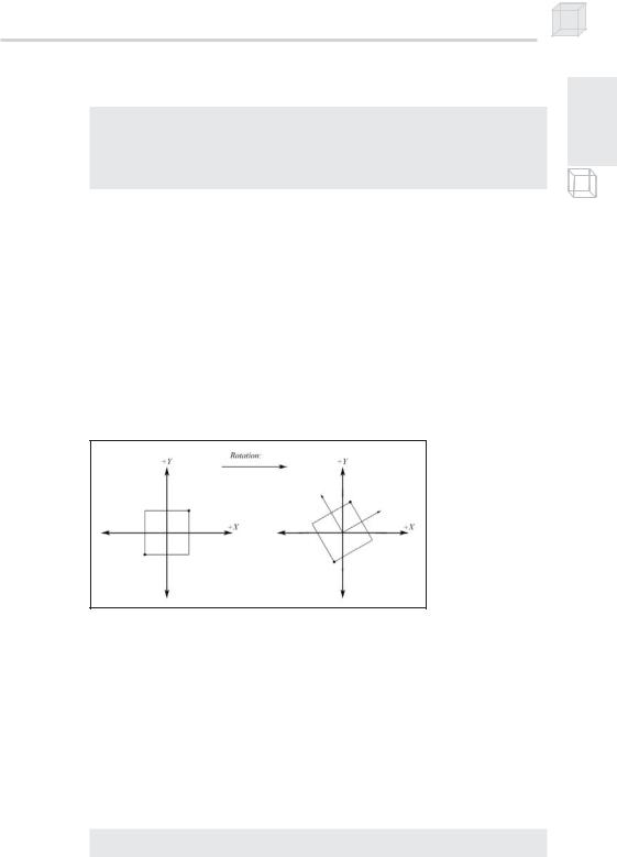
The Rotation Matrices

21

P a r t I

Figure 9: Rotating 30 degrees counterclockwise around the z-axis from our perspective

We can rotate a vector radians around the x-, y-, and z-axis using the following matrices. Note that angles are measured clockwise when looking down the axis of rotation toward the origin.

1	0	0	0
	cos	sin
X 0			0
0	sin	cos	0
0	0	0	1

The D3DX function to build an x-axis rotation matrix is:

D3DXMATRIX *D3DXMatrixRotationX(

D3DXMATRIX* pOut,

// Result.

22 Part I

FLOAT Angle				// Angle of rotation measured in radians.
);
cos		0	sin	0
Y	0	1	0	0
sin		0	cos	0
	0	0	0	1

The D3DX function to build a y-axis rotation matrix is:

D3DXMATRIX *D3DXMatrixRotationY(

D3DXMATRIX* pOut,				// Result.
FLOAT Angle				// Angle of rotation measured in radians.
);
cos		sin	0	0
Z sin		cos	0	0
	0	0	1	0
	0	0	0	1

The D3DX function to build a z-axis rotation matrix is:

D3DXMATRIX *D3DXMatrixRotationZ(

D3DXMATRIX* pOut,	// Result.
FLOAT Angle	// Angle of rotation measured in radians.
);

The inverse of a rotation matrix R is its transpose RT = R–1. Such a matrix is said to be orthogonal.

The Scaling Matrix

Figure 10: Scaling by one-half units on the x-axis and two units on the y-axis

We can scale a vector qx units on the x-axis, qy units on the y-axis, and qz units on the z-axis by multiplying a vector with the following matrix:

qx	0		0		0
0	q		0		0
S q		y
0	0		q	z	0
0	0		0		1

Mathematical Prerequisites 23

P a r t I

The D3DX function to build a scaling matrix is:

D3DXMATRIX *D3DXMatrixScaling(

D3DXMATRIX* pOut,	// Result.
FLOAT sx,	// Number of units to scale on the x-axis.
FLOAT sy,	// Number of units to scale on the y-axis.
FLOAT sz	// Number of units to scale on the z-axis.
);

The inverse of a scaling matrix is found by taking the reciprocal of each scaling factor:

								1		0		0		0
								qx
								0		1		0		0
	1		1		1
S 1 S		,		,							qy
qx			qy		qz							1
								0		0				0
													qz
										0		0
								0						1

Combining Transformations

Often we apply a sequence of transformations to a vector. For instance, we may scale a vector, then rotate it, and finally translate it into its desired position.

Example: Scale the vector p = [5, 0, 0, 1] by one-fifth on all axes, then rotate it /4 radians on the y-axis, and finally translate it 1 unit on the x-axis, 2 units on the y-axis, and –3 units on the z-axis.

Solution: Note that we must perform a scaling, a y-axis rotation, and a translation. We set up our transformation matrices S, Ry, T for scaling, rotating, and translating, respectively, as follows:

									1	0		0		0
																		.707			.707	0
									5											0
										1
		1 1 1							0			0		0					0	1	0	0
	S		,		,					5						R y
		5																		0	.707
				5 5								1				4		.707				0
									0	0				0
												5							0	0	0	1
										0		0
								0						1