Part IV - Well productivity estimating methods

Forecasting Production Rate

of a Single Well…

	Porosity	Perm.,	Net	Oil	Oil	GOR,	Skin	Prod rate,
	%	md	pay, m	visc., cp	FVF	m3/m3		bopd
Min	11	1.2	30	2	1.1	20	-7	80
Mean	12	12	50	2.5	1.2	20	-6	2670
Max	13	25	70	3	1.3	20	-5	21000

		Production Rate as a Fuzzy Number						Prod Rate Cum. Distribution Curve
		All input parameters are triangular FNs						(Triassic sandstones)
	1						1.0
Membershipgrade	0.2					distributionCum.	0.8
							0.2
	0.8
	0.6						0.6
	0.4						0.4
	0						0.0
	10	100	1000	10000	100000		100	1000	10000	100000
		Production rate, bopd						Production rate, bopd
15 September 2012										71

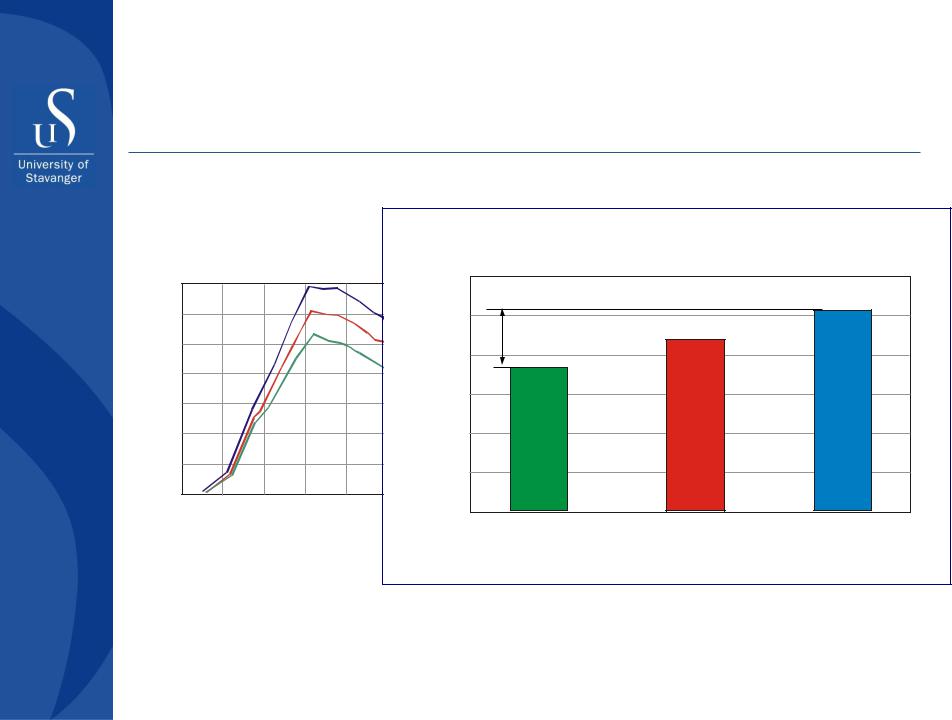
Uncertainty in Production Forecast

				bbl			Uncertainty in cumulative production
					3000
	350			Cumulative production, mill
Production rate, Kbopd
	300				2500
	250				2000		712 mill bbls
	200
	150				1500
	100				1000
	50				500
	0
	0	10	20		30	0	40
			Years				Low	Medium	High
								Scenarios
	15 September 2012								72

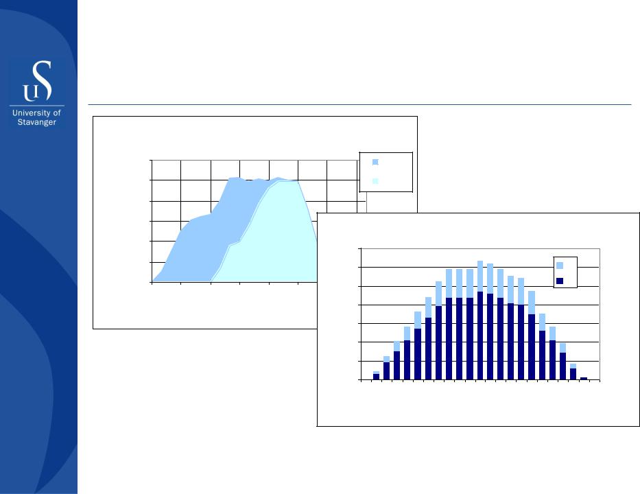
Field-scale Production Forecast

	Contribution of each reservoir into overall
			production
	120									UJ-E
Kbopd
	80
	100									UJ-W
rate,	60										Number of acting wells
prod
	40							70
Oil
	20							60						IW
	0						wells	50						IW
	2016	2019	2022	2025	2028	2031	2034		2037
				Years			of	40
							Number
								30
								20
								10
								0
									2016	2020	2024	2028	2032	2036
Water Cut – 90%												Year

15 September 2012

73

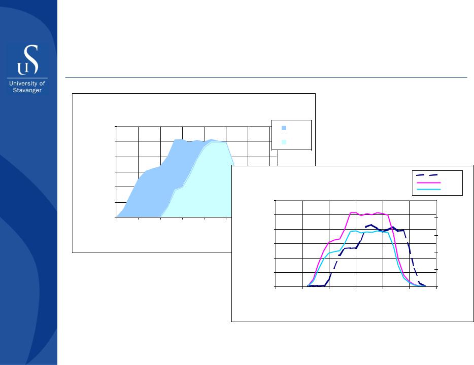
Field-scale Production Forecast

Contribution of each reservoir into overall production

	120									UJ-E
Kbopd	100									UJ-W
	80
rate,	60										Production forecast				Water
Oil prod
	40														Oil
															Gas
	20							120							100
	0							100							80	rate, MMscf/d
	2016	2019	2022	2025	2028	2031	2034		2037
							Kbopdrate,	80							60
				Years
								60
															40
							Oil prod	40								Gas prod
								20							20
								0							0
Water Cut – 90%								2010		2015	2020	2025	2030	2035	2040
												Years
15 September 2012																74

Field-scale Production Forecast

		Reservoir 1	Reservoir 2	Total	Comments
STOOIP, MM STB		1193	892	2085
Area, кm2		200	220	220
Oil recovery, %		22.9	22.7	22.8
Reserves, MM STB		272.7	202.6	475.3
Production plateau, Kbopd		100	66.6	100
Max rate of production (per		13.3	12.0	7.7
year), %
Number of wells:	Prod	50*	50	50	* Recompleted
	Inj	17*	17	17	from the lower
	Total	67*	67	67	reservoir
Area per PW, кm2		4.0	4.0	4.0
STOOIP/PW, MM STB		23.9	17.8	41.7
Initial well production rate, bopd		4442*	3314*	N/A	HW 250 m
Reserves /PW, MM STB		5.45	4.05	9.51
Max watercut, %		90	90	90
Min bottomwhole pressure, bar		291	294	291
Number of the drilling platforms		2M	2M	2M	M (S)– mobile
required					(stationary) unit
Duration of production, years		15	14	21

15 September 2012

75

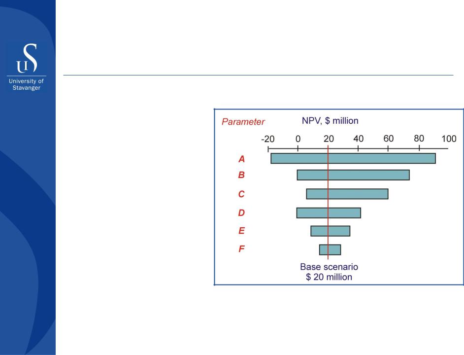
Sensitivity Analysis

The main idea – to identify parameters which uncertainty most influences the project value

Tornado diagram illustrates dependency of the project value on parameter’s uncertainty

15 September 2012

76

Transient

Pressure

Analysis

September 15, 2012	Part IV - Modern well stimulation	77
	methods (Gubkin - IFP program)

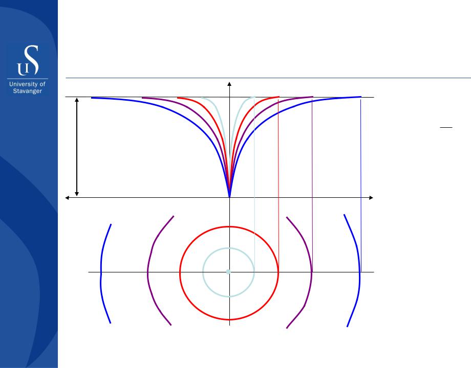
Production Rate Decline Analysis

Reservoir pressure, pe

p pe pwf

Flowing well pressure, pwf Radius, r

Well

re (t) a t

k / o Ct

q(t)		2 kh p
			re (t)
	B ln			S
			rw

September 15, 2012	Part IV - Modern well stimulation	78
	methods (Gubkin - IFP program)

Transient Pressure Analysis

Horizontal well

In transient flow case pressure p(x,y,z,t) should satisfy the following equation:

2 p 2 p 2 p 2 p 1 p x2 y 2 z 2 t

		k
		ct

September 15, 2012	Part IV - Modern well stimulation	79
	methods (Gubkin - IFP program)

Transient Pressure Analysis

Horizontal well

Applying the same method of images for the no cross-flow boundary conditions at the reservoir top and bottom and satisfying a constant wellbore pressure conditions the following equation for a transient pressure flow caused by an arbitrary well can be written:

(x x )2

( y y )2 z jh 1 j z

2

i

i

i

qi erfc

n

4 t

B

p(x, y, z, t)

C

4k

2

2

j

2

j i n

(x xi ) ( y yi ) z jh 1

zi

September 15, 2012	Part IV - Modern well stimulation	80
	methods (Gubkin - IFP program)