

Part IV - Well productivity estimating methods
.pdfTransient Pressure Analysis
Horizontal well
Analysis of transient flow solutions. Flow transformations
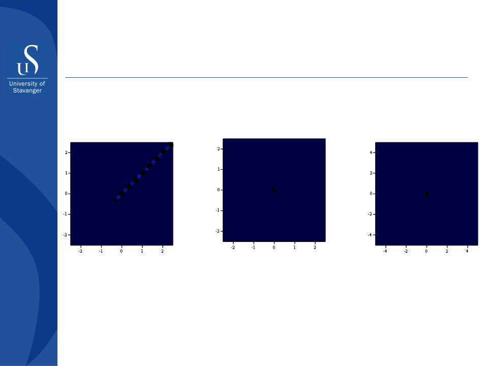
Let’s consider the simplest possible case – one spherical well located in centre (0,0,0) drains reservoir with constant rate q. In that case transient pressure solution becomes:
|
|
|
|
|
|
|
|
|
|
|
|
|
|
|
r 2 jh 2 |
|
|||
|
|
|
erfc |
|
|
|
|
|
|
|
|
|
|
|
4 t |
||||
|
Bq |
|
|
|
|
|
|
||
p(r, t) |
|
|
|
|
|
|
|
|
|
|
|
|
|
|
|
|
|
||
4 k |
|
r 2 jh 2 |
|
|
|||||
|
j |
|
|
|
|||||
September 15, 2012 |
Part IV - Modern well stimulation |
81 |
|
methods (Gubkin - IFP program) |
|

Transient Pressure Analysis
Horizontal well
Analysis of transient flow solutions. Flow transformations
Successful approximation of solution showed that for r/h>0.5 it converges (Fig. 6) to a well known solution for radial flow:
|
Bq |
|
r |
2 |
|
|
f (r, ) |
Ei |
|
|
|||
|
|
|
|
|||
|
4kh |
|
4 t |
|||
It means, that successful application of the well modeling technique (method of images) mathematically proved flow regime transformation: spherical flow between two non-flow boundaries transforms into radial flow
(mathematically, erfc→Ei)
September 15, 2012 |
Part IV - Modern well stimulation |
82 |
|
methods (Gubkin - IFP program) |
|

Transient Pressure Analysis
Horizontal well
Analysis of transient flow solutions. Flow transformations
The same analysis was applied for fully penetrated vertical well. In that case transient pressure solution is equal to:
|
|
|
|
|
|
|
|
|
|
|
|
|
|
|
|
|
|
|
|
|
|
|
j |
2ir |
2 |
|
|||
|
|
|
|
|
|
|
r 2 jh 1 |
|
|
|
||||
|
|
|
erfc |
|
|
|
|
|
|
w |
|
|
|
|
|
|
n |
|
|
|
4 t |
|
|
|
|
|
|||
|
Bq |
|
|
|
|
|
|
|
|
|
|
|||
p(r, t) |
|
|
|
|
|
|
|
|
|
|
|
|
||
4 k |
|
|
|
|
|
|
|
|
|
|
|
|
||
|
|
|
|
|
|
|
|
2 |
|
|
|
|||
|
j i n |
|
|
|
|
|
|
|
|
|
|
|
||
|
|
r |
2 |
jh 1 |
j |
2irw |
|
|
|
|||||
|
|
|
|
|
|
|
|
|
|
|
||||
September 15, 2012 |
Part IV - Modern well stimulation |
83 |
|
methods (Gubkin - IFP program) |
|

Transient Pressure Analysis
Horizontal well
Analysis of transient flow solutions. Flow transformations
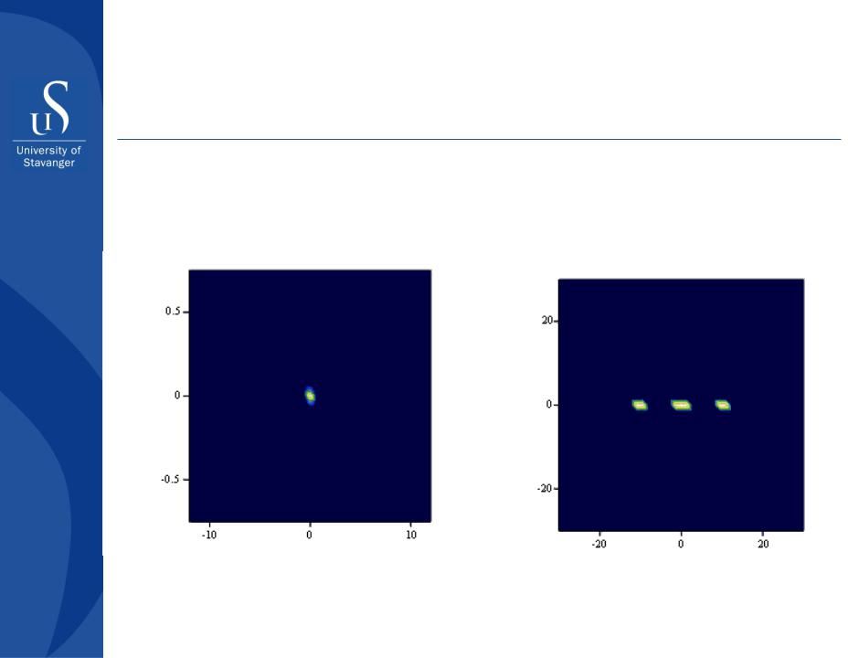
Continuing with flow regime transformation we have applied the same method of images for a fully penetrated vertical well located in the middle of a (sand) channel between two non-permeable boundaries. In this case pressure solution becomes:
|
|
|
|
|
|
|
|
|
|
|
|
Bq |
|
|
r |
2 |
( jD) |
2 |
|
||
f (r,t) |
Ei |
|
|
|||||||
|
|
|
|
|
|
|
|
|||
4 kh |
|
|
4 t |
|
|
|||||
|
j |
|
|
|
|
|
|
|||
September 15, 2012 |
Part IV - Modern well stimulation |
84 |
|
methods (Gubkin - IFP program) |
|

Transient Pressure Analysis
Horizontal well
Analysis of transient flow solutions. Flow transformations
Successful approximation of solution showed that for r/D>0.5 it converges to the linear flow solution:
|
|
|
|
|
r 2 |
|
|
|
|
|
|
|
|
|
|
|
|
|
Bq |
|
|
|
|
|
Bqr |
|
|
r |
|
|
|||
|
|
4 |
t |
|
|
|
|
|
||||||||
l(r, ) |
|
|
|
e |
|
|
|
|
|
|
erfc( |
|
|
|
|
) |
|
|
|
|
|
|
|
|
|
|
|
||||||
kh D |
|
|
|
2khD |
t |
|||||||||||
2 |
|
|
|
|
|
2 |
|
|
||||||||
The latter example proves another flow regime transformation: radial flow between two non-flow boundaries converges into a linear flow (mathematically Ei→exp-erfc)
September 15, 2012 |
Part IV - Modern well stimulation |
85 |
|
methods (Gubkin - IFP program) |
|

Transient Pressure Analysis
Horizontal well
September 15, 2012 |
Part IV - Modern well stimulation |
86 |
|
methods (Gubkin - IFP program) |
|
Transient Pressure Analysis
Slant well
September 15, 2012 |
Part IV - Modern well stimulation |
87 |
|
methods (Gubkin - IFP program) |
|
Transient Pressure Analysis
9 production horizontal wells in grid
September 15, 2012 |
Part IV - Modern well stimulation |
88 |
|
methods (Gubkin - IFP program) |
|

Reservoir Simulation and
Production Forecasting
Methods
15 September 2012 |
89 |
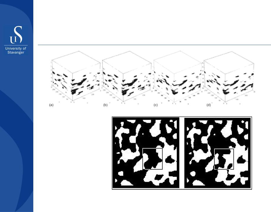
Reservoir characterization / geomodeling
Extracted from Pourpak et al., 2009
Extracted from Kretz et al., 2002
15 September 2012 |
90 |