Добавил:

fench Опубликованный материал нарушает ваши авторские права? Сообщите нам.

Вуз:

Сумский государственный университет

Предмет:

Биомеханика

Файл:

Wiley - Encyclopedia of Medical Devices and Instrumentation - Vol. 3.pdf

Скачиваний:

296

Добавлен:

10.08.2013

Размер:

16.56 Mб

Скачать

☆

<<< < Предыдущая 1 2 3 4 5 6 7 89 / 469 10 11 12 13 14 15 16 17 18 19 20 21 22 23 24 25 > Следующая >>>

62ELECTROENCEPHALOGRAPHY

57.Rasmussen KG, Jarvis MR, Zorumski CF, Ruwitch J, Best AM. Low-dose atropine in electroconvulsive therapy. J ECT 1999;15(3):213–221.

58.McCall WV. Antihypertensive medicines and ECT. Convulsive Ther 1993;9:317–325.

59.Nishihara F, Ohkawa M, Hiraoka H, Yuki N, Saito S. Beneﬁts of the laryngeal mask for airway management during electroconvulsive therapy. J ECT 2003;19:211–216.

60.Brown NI, Mack PF, Mitera DM, Dhar P. Use of the ProSealTM laryngeal mask airway in a pregnant patient with a difﬁcult airway during electroconvulsive therapy. Br J Anaesthesia 2003;91:752–754.

61.Sackeim HA. The anticonvulsant hypothesis of the mechanism of action of ECT: Current status. J ECT 1999;15(1):5–26.

62.Sackeim HA, Long J, Luber B, Moeller J, Prohovnik I, Davanand DP, Nobler MS. Physical properties and quantiﬁcation of the ECT stimulus: I. Basic principles. Convulsive Ther 1994;10(2):93–123.

63.Abrams R, Swartz CM. Thymatron1 System IV Instruction Manual. 8th ed. Somatics, LLC; 2003.

64.Sackeim HA, Prudic J, Devanand DP, Kiersky JE, Fitzsimons L, Moody BJ, McElhiney MC, Coleman EA, Settembrino JM. Effects of stimulus intensity and electrode placement on the efﬁcacy and cognitive effects of electroconvulsive therapy. N Engl J Med 1993;328:839–846.

65.Delva NJ, Brunet D, Hawken ER, Kesteven RM, Lawson JS, Lywood DW, Rodenburg M, Waldron JJ. Electrical dose and seizure threshold: Relations to clinical outcome and cognitive effects in bifrontal, bitemporal, and right unilateral ECT. J ECT 2000;16:361–369.

66.Bailine SH, Rifkin A, Kayne E, Selzer JA, Vital-Herne J, Blieka M, Pollack S. Comparison of bifrontal and bitemporal ECT for major depression. Am J Psychiatry 2000;157:121– 123.

67.Letemendia FJJ, Delva NJ, Rodeburg M, Lawson JS, Inglis J, Waldron JJ, Lywood DW. Therapeutic advantage of bifrontal electrode placement in ECT. Psycholog Med 1993;23:349– 360.

68.Lawson JS, Inglis J, Delva NJ, Rodenburg M, Waldron JJ, Letemendia FJJ. Electrode placement in ECT: Cognitive effects. Psycholog Med 1990;20:335–344.

69.Benbadis S. Epileptic seizures and epileptic syndromes. Neurolog Clin 2001;19(2):251–270.

70.Beyer JL, Weiner RD, Glenn MD. Electroconvulsive Therapy: A Programmed Text. 2nd ed. Washington (DC): American Psychiatric Press; 1985.

71.Petrides G, Fink M. The ‘‘half-age’’ stimulation strategy for ECT dosing. Convulsive Ther 1996;12:138–146.

72.Newman ME, Gur E, Shapira B, Lerer B. Neurochemical mechanisms of action of ECT: Evidence from in vivo studies. J ECT 1998;14(3):153–171.

73.Mann JJ. Neurobiological correlates of the antidepressant action of electroconvulsive therapy. J ECT 1998;14(3):172– 180.

74.Sanacora G, Mason GF, Rothman DL, Hyder F, Ciarcia JJ, Ostroff RB, Berman RM, Krystal JH. Increased cortical GABA concentrations in depressed patients receiving ECT. Am J Psychiatry 2003;160(3):577–579.

75.Nobler MS, Teneback CC, Nahas Z, Bohning DE, Shastri A, Kozel FA, Goerge MS. Structural and functional neuroimaging of electroconvulsive therapy and transcranial magnetic stimulation. Depression Anxiety 2000;12(3):144–156.

76.Nobler MS, Oquendo MA, Kegeles LS, Malone KM, Campbell CC, Sackeim HA, Mann JJ. Decreased regional brain metabolism after ECT. Am J Psychiatry 2001;158(2):305–308.

77.Drevets WC. Functional neuroimaging studies of depression: The anatomy of melancholia. Annu Rev Med 1998;49:341–361.

78.Nobler MS, Sackeim HA, Prohovnik I, Moeller JR, Mukherjee S, Scnur DB, Prudic J, Devanand DP. Regional cerebral blood ﬂow in mood disorders, III. Treatment and clinical response. Arch Gen Psychiatry 1994;51:884–897.

79.George MS, Nahas Z, Li X, Kozel FA, Anderson B, Yamanaka K, Chae J-H, Foust MJ. Novel treatments of mood disorders based on brain circuitry (ECT, MST, TMS, VNS, DBS). Sem Clin Neuropsychiatry 2002;7:293–304.

80.Duman RS, Vaidya VA. Molecular and cellular actions of chronic electroconvulsive seizures. J ECT 1998;14(3):181–193.

81.George MS, Nahas Z, Kozel FA, Li X, Denslow S, Yamanaka K, Mishory A, Foust MJ, Bohning DE. Mechanisms and state of the art of transcranial magnetic stimulation. J ECT 2002;18: 170–181.

Reading List

Abrams R. Electroconvulsive Therapy. 4th ed. New York: Oxford University Press; 2002.

Sackeim HA, Devanand DP, Nobler MS. Electroconvulsive therapy. In: Bloom FE, Kupfer DJ, editors. Psychopharmacology: The Fourth Generation of Progress. 4th ed. New York: Raven Press; 1995.

Rasmussen KG, Sampson SM, Rummans TA. Electroconvulsive therapy and newer modalities for the treatment of medicationrefractory mental illness. Mayo Clin Proc 2002;77:552–556.

Dolenc TJ, Barnes RD, Hayes DL, Ramussen KG. Electroconvulsive therapy in patients with cardiac pacemakers and implantable cardioverter deﬁbrillators. PACE 2004;27:1257–1263.

Electroconvulsive Therapy. NIH Consensus Statement, June 10– 12, 1985, National Institutes of Health, Bethesda, MD Online. Available at http://odp.od.nih.gov/consensus/cons/051/ 051_statement.htm.

Information about ECT. New York State Ofﬁce of Mental Health. Online. Available at http://www.omh.state.ny.us/omhweb/ect/ index.htm. and http://www.omh.state.ny.us/omhweb/spansite/ ect_sp.htm (Spanish version).

See also ELECTROENCEPHALOGRAPHY; REHABILITATION, COMPUTERS IN COGNITIVE.

ELECTRODES. See BIOELECTRODES; CO2 ELECTRODES.

ELECTROENCEPHALOGRAPHY

DAVID SHERMAN

DIRK WALTERSPACHER

The Johns Hopkins University

Baltimore, Maryland

INTRODUCTION

The following section will give an overview of the electroencephalogram (EEG), its origin, and its validity for diagnosis in clinical use. Since Berger (1) demonstrated in 1929 that the activity of the brain can be measured using external electrodes placed directly on the intact skull, the EEG has been used to study functional states of the brain. Although the EEG signal is the most common indicator for brain injuries and functional brain disturbances, the complicated underlying process, creating the signal, is still not well understood.

ELECTROENCEPHALOGRAPHY 63

The section is organized as follows. The biophysical basis of the origin of the EEG signal is described ﬁrst, followed by EEG recordings and classiﬁcation. Afterward, the validity and scientiﬁc basis for using the EEG signal as a tool for studying brain function and dysfunction is presented. Finally, logistical and technical considerations as they have to be made in measuring and analyzing biomedical signals are mentioned.

ORIGIN OF EEG

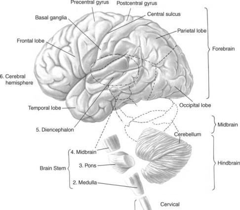
Valid clinical interpretation of the electroencephalogram ultimately rests on an understanding of the basic electrochemical and electrophysical processes through which the patterns are generated and the intimate nature of the brain’s functional organization, at rest and in action. Therefore, the succeeding parts of the following discussion deal with the gross organization of the cortex, which is generally assumed to be the origin of brain electrical activity that is recorded from the surface of the head (2– 4), the different kinds of electrical activity and resulting potential ﬁelds developed by cortical cells. Figure 1 shows the general organization of the human brain.

Organization of the Cerebral Cortex

Even though different regions of the cortex have different cytoarchitectures and each region has its own morphological patterns, aspects of intrinsic organization of the cortex are general (6,7). Most of the cortical cells are

Figure 1. The major portions of the human cerebrum called lobes. Areas external to the cerebrum include the midbrain areas such as the diencephalon and the hindbrain areas such as the cerebellum, medulla, and pons. (Adapted from Ref. 5.)

arranged in the form of columns, in which the neurons are distributed with the main axes of the dendritic trees parallel to each other and perpendicular to the cortical surface. This radial orientation is an important condition for the appearance of powerful dipoles. Figure 2 shows the schematic architecture of a cortical column. It can be observed that the cortex, and within any given column, consist of different layers. These layers are places of specialized cell structures and within places of different functions and different behaviors in electrical response. An area of very high activity is, for example, layer IV, which neurons function to distribute information locally to neurons located in the more superﬁcial (or deeper) layers. Neurons in the superﬁcial layers receive information from other regions of the cortex. Neurons in layers II, III, V, and VI serve to output the information from the cortex to deeper structures of the brain.

Activity of a Single Pyramidal Neuron

Pyramidal neurons constitute the largest and the most prevalent cells in the cerebral cortex. Large populations of these pyramidal neurons can be found in layers IV and V of the cortex. EEG potentials recorded from electrodes placed on the scalp represent the collective summation of changes in the extracellular potentials of pyramidal cells (2–4).

The pyramidal cell membrane is never completely at rest because it is continually inﬂuenced by activity arising in other neurons with which it has synaptic connections (8).

64 ELECTROENCEPHALOGRAPHY

Figure 2. Schematic of the different layers of the cerebral cortex. Pyramidal cells that are mainly in layers III and V are mainly responsible for the generation of the EEG. (Adapted from Ref. 5.)

Such synaptic connections may be excitatory or inhibitory and the respective transmitter changes the permeability of the membrane for Kþ (and/or Cl ), which results in a ﬂow of current (for details, please see Ref. 8).

The ﬂow of current in response to an excitatory postsynaptic potential at the site on the apical dendrite of a cortical pyramidal neuron is shown in Fig. 3. The excitatory postsynaptic potential (EPSP) is associated with an inward current at the postsynaptic membrane carried by positive ions and an outward current along the large expanse of the extra-synaptic membrane. For simplicity, only one path of outward current is illustrated through the soma membrane. This current ﬂow in the extracellular space causes the generation of a small potential due to extracellular resistance (shown by R in Fig. 3).

As an approximation it is possible to estimate the extracellular ﬁeld potential as a function of the transmembrane potential (9)

	a2s	Z	@2vm=@x2
fe ¼	i			dx	ð1Þ
	4se		r

where fe is the extracellular potential, a is the radius of axon or dendrites, vm is the transmembrane potential, si, is the intracellular conductance, and se is the extracellular conductance. For a derivation of the above mentioned equation, please see Ref. 9.

Although these extracellular potentials individually are small, their sum becomes signiﬁcant when added over many of cells. This is because the pyramidal neurons are more or less simultaneously activated by this way of synaptic connections and the longitudinal components of their extracellular currents will add, whereas their transversal components will tend to cancel out.

Figure 3. The current ﬂow within a large pyramidal cell. Ionic ﬂow is established to enable charge balance. (Adapted from Ref. 2.)

Generation of EEG Potentials

The bulk of the gross potentials recorded from the surface of the scalp results from the extracellular current ﬂow associated with summated postsynaptic potentials in synchronously activated vertically oriented cortical pyramidal neurons. The exact conﬁguration of the gross potential is related in a complex fashion to the site and the polarity of the postsynaptic potentials. Considering two cortical pyramidal neurons (shown in Fig. 3), the potential measured by a microelectrode at the location P is given by (4)

	1			Ia				Ia
F pðtÞ ¼					cosð2p fat þ aaÞ				cosð2p fat þ aaÞ
	4ps			R1				R2
		Ib				Ib
	þ		cosð2p fbt þ abÞ				cosð2p fbt þ abÞ
		R3				R4

þ Similar contributions from other dipoles ð2Þ

where Ia and Ib are the peak magnitudes of current for each dipole with phases aa and ab, respectively, and is the conductivity of the medium. ‘‘Similar contribution from other dipoles’’ refers to the contribution of dipoles other than the two shown, most signiﬁcantly from the dipoles physically close to the electrode. Dipoles that are farther from the recording electrode but in synchrony (aa ¼ ab ¼

. . . ¼ a), and aligned in parallel, contribute an average potential proportional to the number of synchronous dipoles jFpj m. Dipoles that are either randomly oriented or with a random phase distribution contribute an average

potential proportional to the square root of their number p

Fpj m. Thus, the potential measured by a microelectrode can be expressed by the following approximate relation (4):

Isd

Iad

Fpj

þ m

þ n

ð3Þ

8ps

Rs2

Ra2

i¼1

Here the subscripts i s, and a refer to local, remote synchronous, and remote asynchronous dipoles. Is And Ia are the effective currents for remote synchronous and remote asynchronous sources, which may be less than the total current, depending on the orientation of the sources with respect to the electrode. Also l, m, and n are the numbers of local, remote synchronous, and remote asynchronous sources, which are located at average distances Ri, Rs, and Ra respectively. Note that a microelectrode like the scalp electrode used for EEG recordings measures a ﬁeld averaged over a volume large enough to contain perhaps 107–109 neurons.

Contribution of Other Sources

A decrease in the membrane potential to a critical level of approximately 10 mV less than its resting state (depolarization) initiates a process that is manifested by the action potential (10). Although it might seem that action potentials traveling in the cortical neurons are a source of EEG, they contribute little to surface cortical records, because they usually occur asynchronously in time in large numbers of axons, which run in many directions relative to the surface. Other reasons are that the piece of membrane that is depolarized by an action potential at any instant of time

ELECTROENCEPHALOGRAPHY 65

is small in comparison with the portion of membrane activated by an EPSP and that action potentials are of short durations (1–2 ms) in comparison with the duration of EPSPs or IPSPs (10–250 ms). Thus, their net inﬂuence on potential at the surface is negligible. An exception occurs in the case of a response evoked by the simultaneous stimulation of a cortical input (11), which is generally called a compound action potential.

Other cells in the cortex like the glial cells are unlikely to contribute substantially to surface records because of their irregular geometric organization, such that produced ﬁelds of current ﬂow sum to a small value when viewed from a relatively great distance on the surface. There is also activity in deep subcortical areas, but the resulting potentials are too much attenuated at the surface to be recordable.

The discussed principles show that the surface-recorded EEG can be observed as the result of many active elements, where the postsynaptic potentials from cortical pyramidal cells are the dominant source.

Volume Conduction of EEG

Recording from the scalp has the disadvantage that there are various layers with different conductivities between the electrode and the area of cortical potential under the electrode. Therefore, potentials recorded at the scalp are not only inﬂuenced by the above mentioned patterns, but also by regions with different conductivities. Layers lying around the brain are such regions. These include the cerebrospinal ﬂuid (CSF), the skull, and the scalp. These layers account, at least in part, for the attenuation of EEG signals measured at the surface of the scalp, as compared with those recorded with a microelectrode at the underlying cortical surface or with a grid of electrodes directly attached to the cortex (ECoG). These shells surrounding the brain account for an attenuation factor of 10 to 20 (12). This attenuation mainly affects the high-frequency–low- voltage component (the frequency range above 40 Hz), which has been shown to carry important information about the functional state of the brain, but it is almost totally suppressed at the surface.

EEG SIGNAL

The EEG signal consists of spontaneous potential ﬂuctuations that also appear without a sensory input. It seems to be a stochastic signal, but it is also composed of quasisinusoidal rhythms. The synchrony of cerebral rhythms may occur from pacemaker centers in deeper cortical layers like the thalamus or in subcortical regions, acting through diffuse synaptic linkages, reverberatory circuits incorporating axonal pathways with extensive ramiﬁcations, or electrical coupling of neuronal elements (13). The range of amplitudes is normally from 10 to 150 mV, when recorded from electrodes attached to the scalp. The EEG signal consists of a clinical relevant frequency range of 0.5–50 Hz (10).

EEG Categories

Categorizing EEG signals into waves of a certain frequency range has been used since the discovery of the electrical

66 ELECTROENCEPHALOGRAPHY

Figure 4. (a) Examples of EEG from different frequency bands. (b) The phenomenon of alpha desynchronization. (From Ref. 14).

activity of the brain. Therefore, these different frequency bands have been the most common feature in EEG analysis. Although this feature contains a lot of useful information as presented below, its use is not with criticism. It can be observed that there is some physiological and statistical evidence for the independence of these bands, but the exact boundaries vary between people and change with the behavioral state of each person (age, mental state, etc.). In particular, between human EEG and EEG signals recorded from different species of animals one can ﬁnd different EEG patterns and frequency ranges. Nevertheless, the different frequency bands for human EEG are described below, because of their importance as an EEG feature. Most of the patterns observed in human EEG could be classiﬁed into one of the following bands or ranges:

Delta	below 3.5 Hz (usually 0.1–3.5 Hz)
Theta	4–7.5 Hz
Alpha	8–13 Hz
Beta	usually 14–22 Hz

A typical plot of these frequency bands is shown in Fig. 4, and the different bands are described below.

Delta Waves. The appearance of delta waves is normal in neonatal and infants’ EEGs and during sleep stages in adult EEGs. When slow activity such as the delta band appears by itself, it indicates cerebral injury in the waking adult EEG. Dominance of delta waves in animals that have had subcortical transections producing a functional separation of

cerebral cortex from deeper brain regions suggests that these waves originate solely within the cortex, independent of any activity in the deeper brain regions.

Theta Waves. This frequency band was included in the delta range until Walter and Dovey (15) felt that an intermediate band should be established. The term ‘‘theta’’ was chosen to allude to its presumed thalamic origin.

Theta frequencies play a dominant role in infancy and childhood. The normal EEG of a waking adult contains only a small amount of theta frequencies, mostly ovserved in states of drowsiness and sleep. Larger contingents of theta activity in the waking adult are abnormal and are caused by various forms of pathology.

Alpha Waves. These rhythmic waves are clearly a manifestation of the posterior half of the head and are usually found over occipital and parietal regions. These waves are best observed under conditions of awakeness but during physical relaxation and relative mental inactivity. The posterior alpha rhythm can be temporarily blocked by mental activities, or afferent stimuli such as inﬂux of light while eye opening (Fig. 4b). This alpha blocking response was discovered by Berger in 1929 (1). Mainly thalamocortical feedback loops are believed to play a signiﬁcant role in the generation of the alpha rhythm (16).

Beta Waves. Beta activity is found in almost every healthy adult and is encountered chieﬂy over the frontal and central regions of the cortex. The voltage is much lower than in alpha activity (seldom exceeds 30 mV). Beta

ELECTROENCEPHALOGRAPHY 67

		Vertex	Front
FZ	20%	CZ
FZ		CZ	20%
			20%

20%

FP1

FP2

FP1

20%

10%

Nasion

Pg1

10% Left

Right

Inion

Side

Ear

Back

Figure 5. (a)and (b) The side and top view of the layout of a standardized 10–20 electrode system. Adapted from Ref. 14.

activity shows considerable increase in quantity and voltage after the administration of barbiturates, some nonbarbituric sedatives, and minor tranquilizers. It also appears during intense mental activity and tension.

Clinical EEG

To obtain EEG recordings, there are several standardized systems for electrode placement on the skull. The most common are those of the standard 10–20 system of the International EEG Federation, which uses 30 electrodes placed on four landmarks of the skull as observed in Fig. 5.

It is now possible to obtain unipolar (or monopolar) and bipolar derivations from these electrodes. Using a bipolar derivation, one channel is connected between a pair of electrodes and the resultant difference in the potential between these two electrodes is recorded. Therefore, bipolar derivations give an indication of the potential gradient between two cerebral areas. Unipolar (monopolar) derivations can either be obtained by recording the potentialdifference between the ‘‘active’’ electrodes and one ‘‘indifferent’’ electrode, placed elsewhere on the head (ear, nose), or with respect to an average reference, by connecting all other leads through equal-valued resistances (e.g., 1 MV) to a common point (17). The advantages of unipolar derivations are that the amplitude of each deﬂection is proportional to the magnitude of the potential change that causes it and the demonstration of small time differences between the occurrence of a widespread discharge at several electrodes. Small, nonpolarizable, disk Ag-AgCl electrodes are used together with an electrode paste. Recorded potentials are ampliﬁed using a high gain, differential, capacitivly coupled ampliﬁer. The output signals are displayed on a chart recorder or a monitor screen. For more details about unipolar or bipolar derivations and EEG-ampliﬁers, please see (Ref. 11).

SCIENTIFIC BASIS FOR EEG MONITORING

The scientiﬁc basis for using EEG as a tool for studying brain function and dysfunction rests on the following four neurobiologic qualities of EEG.

Link With Cerebral Metabolism

The above presented discussion on the origin of potentialdifferences, recorded from the brain, shows that the EEG can be observed as a result of the synaptic and cellular activity of cortical pyramidal neurons. These neuronal and synaptic activities are directly linked to cerebral metabolism. Cerebral metabolic activity in turn depends on multiple factors including enzyme synthesis, substrate phosphorylation, axonal transport, and adenosine triphosphate (ATP) production from mitochondrial and glytolytic pathways (18). Thus, the EEG is a composite phenomenon reﬂecting complicated intracellular, intraneuronal, and neuro-glial inﬂuences. Although this multifaceted system makes it obvious that a selection of any single mechanism underlying the electrocortical manifestations may not be possible, the EEG is still a highly sensitive indicator of cerebral function (19).

Sensitivity to Most Common Causes of Cerebral Injury

The most common causes of cerebral injury are hypoxia and ischemia. It can be observed that hypoxia-ischemia causes a severe neuronal dropout in the cortical layers 3 and 5, leading to well-known hisyophatologic patterns of laminar necrosis. As pyramidal neurons that occupy the cortical layers are the main source for EEG, this loss of neuronal activity changes the cortical potentials and therefore makes EEG very sensitive to these common insults.

Correlation With Cerebral Topography

The standardized systems for electrode placement (Jung, international 10–20 system, etc.) establish a consistent relationship between electrode placement and underlying cerebral topography (20). Therefore, changes in EEG recorded from these electrodes of different areas of the skull reﬂect a consistent topographical relationship with underlying cerebral structures and allows useful inferences about disease localization from abnormalities in EEG detected at the scalp.

68 ELECTROENCEPHALOGRAPHY

Ability to Detect Dysfunctions at a Reversible Stage

Heuser and Guggenberger (21) showed in 1985 that EEG deteriorates before the disruption of neuronal membrane and before signiﬁcant reduction of cellular ATP levels. Siesjo and Wieloch (22) demonstrated in 1985 that during cerebral ischemia, changes in EEG correlate with elevated tissue lactate levels while ATP levels remain normal. Astrup (23) showed that a reduction in cerebral blood ﬂow (CBF) affects EEG much before it causes neuronal death. These and several other reports make it clear that EEG offers the ability to detect injury at a reversible stage.

EEG also allows a prediction of recovery after brain dysfunctions like cerebral ischemia after cardiac arrest (24). Various studies in this report show that EEG recordings at several stages during recovery allow the prediction of whether the patient has a favorable outcome. Goel (25) showed that parameters obtained from EEG recordings may serve as an indicator for the outcome after hypoxicasphyxic encephalophaty (HAE). These attributes make the EEG a very attractive neurologic observational tool.

LOGISTICAL AND TECHNICAL CONSIDERATIONS

Although the last sections have shown that EEG signal detection may serve as an important indicator for detection of neurological status and disorders, its clinical use and acceptance under a neurological care regime is limited. This is due to the complicated nature of the EEG signal and because of the difﬁculties regarding the interpretation of the signals. Some challenges of EEG analysis are as follows.

Artifacts

Recordings of physiological signals, especially from the surface of the body, have the problem that they are superimposed or distorted by artifacts. EEG signals are especially prone to artifact distortions due to their weak character. Therefore, a knowledge about the possible sources of distortion is necessary to estimate the signal-to-noise ratio (SNR). These artifacts are mostly generated from various kinds of sources. The sources of artifacts can be devided into two mayor groups: the subject-generated artifacts and the artifacts generated by the equipment. Subject-generated artifacts include EMG artifacts like body movement, muscle contraction of the neck, chewing, swallowing, coughing, involuntary movements (like myoclonic jerks, palotal myoclonus, nystagmus, asymmetric oculomotor paralysis, and decerebrate or decorticate posturing), and eye movements. Scalp edema can produce artifactual reductions in amplitude regionally or over an entire hemisphere. Pulse and EKG could also contribute as artifacts in EEG.

Artifacts generated by the equipment include ventilator artifacts that typically appear as slow wave like activity, vibrations of electrical circuitry around the subject, and power line interference. By taking the appropriate methods, a lot of these artifacts can be prevented [for more details, see Mayer-Waarden (10)].

Another method, to eliminate both artifacts generated by the equipment and the subject, is to use a differential ampliﬁer for the recording between two electrodes. The

assumption here is that the transmission time of artifacts between two electrodes can be neglected, and therefore, the artifacts at both electrodes are in-phase. The signal to be recorded is assumed to have a time delay from one to another electrode, and taking the difference therefore eliminates the artifact but keeps the signals’ nature.

Inter-User Variability

Interpreting physiological signals is difﬁcult, even for specialists, because of their subject-speciﬁc nature. The complicated nature of EEG signals makes it even more difﬁcult, and data generated by different EEG analysis methods (especially techniques like feature analysis, power spectral analysis, etc.) may be interpreted in different ways by different analysts. An analysis of inter-user-variability of clinical EEG interpretation was presented by Williams et al. (26), which showed that even EEG data interpretation by EEG analysts could be different. Therefore, more standardized and objective methods of EEG analysis are extremely desirable.

Inter-Individual Variability

As mentioned, the consistency of the human EEG is inﬂuenced by many parameters and makes EEG unique for a certain person and for a speciﬁc point-in-time. Intrinsic parameters are the age and the mental state of the subject (degree of wakefulness, level of vigilance), the region of the brain, hereditary factors, and inﬂuences on the brain (injuries, functional disturbances, diseases, stimuli, chemical inﬂuences, drugs, etc.). To detect deviations from ‘‘normal’’ EEG, it would be necessary to compare this ‘‘abnormal’’ EEG with the ‘‘normal’’ EEG as a reference. Therefore, attempts have been made to obtain normative EEG for each of the classes discussed above (i.e, normative EEG for various age groups, normative EEG under the inﬂuence of varying amounts of different drugs, etc.), but these databases of normative data are still not sufﬁcient to cover the variety of situations possible in real-life recordings. On the other hand, these normative data vary too much for considering them as one person’s ‘‘normal’’ EEG.

Labor-Intensive and Storage Problems

For patient monitoring in the operating room or for chronic monitoring tasks that are necessary for cases of gradual insults and injuries, the EEG recordings can be extremely labor intensive. This makes it necessary to have either efﬁcient means of collecting, storing, and displaying the long-term recordings or to come up with new techniques of compressing the EEG data, while preserving its characteristic features. Better methods to overcome these problems have been developed in both directions, although primarily toward efﬁcient storage and display techniques. Methods of compressed spectral array representation overcome the limitation of compressed display to a great extent.

DISCUSSION

The review presented above emphasizes that the EEG is sensitive to different states of the brain and therefore may

serve as a useful tool for neurological monitoring of brain function and dysfunction. In various clinical cases, the EEG has been used to observe patients and to make critical decisions. Nevertheless, its complicated nature and difﬁculty of interpretation has limited its clinical use. The following section should give an overview of the common techniques in analyzing EEG signals.

TECHNIQUES OF EEG ANALYSIS

Introduction

The cases presented above show that EEG has signiﬁcant clinical relevance in detecting several diseases as well as in different stages of recovery. Still the complex nature of EEG has so far restricted its use in many clinical situations. The following discussion should give an overview of the state-of-the-art EEG monitoring and analysis techniques. The presented EEG analysis methods are divided into two basic categories, parametric and nonparametric, respectively, assuming that such a division is conceptually more correct than the more common differentiation between frequency and time-domain methods because they represent two different ways of describing the same phenomena.

NonParametric Methods

In most of these analysis methods, the statistical properties of EEG signals are considered realizations of a Gaussian random process. Thus, the statistics of an EEG signal can be described by the ﬁrst-and second-order moments.

These nonparametric time-domain and frequencydomain methods have been the most common way in analyzing EEG signals. In the following description of the different methods, it is also mentioned whether the technique is still being used in clinical settings.

Clinical Inspection. The most prevalent method of clinically analyzing the EEG is the visual inspection of chart records obtained from EEG machines. It uses the features observed in real-time EEG (like low frequencyhigh amplitude activity, burst suppression activity, etc.) for diagnostic and prognostic purposes. Several typical deviations from the normal EEG are related to different stages of the brain. This method suffers from the limitations like inter-user variability, labor intensiveness, and storage problems. A detailed description of logistical and technical considerations faced with EEG analysis is given later in this section.

Amplitude Distribution. Amplitude distribution is based on the fact that a random signal can be characterized by the distribution of its amplitude and accompanying mean, variance, and higher order moments. It can be observed that the amplitude distribution of an EEG signal most of the time can be considered as Gaussian (27) and the deviations from Gaussianity and its time-varying properties have been clinically used to detect and analyze different sleep stages (28,29). This method is now less popular because of more powerful and sophisticated EEG analysis techniques.

ELECTROENCEPHALOGRAPHY 69

Interval Distribution. This is one of the earliest methods of quantitating the EEG (30). The method is based on measuring the distribution of intervals between either zero or other level crossings, or between maxima and minima. Often, the level crossings of the EEG’s ﬁrst and second derivatives are also computed to obtain more information about the spectral properties of the signal. Due to its ease of computation, the method has been shown to be useful in monitoring long-term EEG changes during anesthesia or sleep stages. Although simple, some theoretical problems are associated with this technique: It is extremely sensitive to high-frequency noise in the estimation of zero crossings and to minor changes in EEG. Also the zero crossing frequency (ZXF), the number of times the EEG signal crosses the zero voltage line, is not unique to a given waveform. Very different waveforms could give rise to the same ZXF. Despite the limitations, modiﬁed versions of period analysis are still used for clinical applications (30).

Interval-Amplitude Analysis. Interval-amplitude analysis is the method by which the EEG decomposed in waves or half-waves, both deﬁned in time, by the interval between zero crossings, and in amplitude by the peak-to-through amplitudes. The amplitude and the interval duration of a half-wave are deﬁned by the peak through differences in amplitude and time; the amplitude and the interval duration of a wave are deﬁned by the mean amplitude and the sum of the interval durations of two consecutive half-waves (31,32). This method has been used clinically for sleep monitoring and depth of anesthesia studies (33).

Correlation Analysis. The computation of correlation functions constituted the forerunner of contemporary spectral analysis of EEG signals (34,35). The correlation function for random data describes the general dependence of the values of the data at one time on the values of the same data in the case of autocorrelation analysis (or of different data in the case of cross-correlation analysis) at another time. The cross-correlation between two signals x and y is deﬁned as

FxyðtÞ :¼ EfxðtÞyðt þ tÞg

ð4Þ

where t is the lag time (note that Fxy(t) becomes the autocorrelation function for x ¼ y and it can be estimated for discrete data by

^	1		Njmj1
FxyðmÞ ¼			X	xðnÞyðn þ mÞ;
FxyðmÞ ¼		N jmj	n 0	xðnÞyðn þ mÞ;
			¼		ð5Þ
	m ef0; 1; 2; : . . . ; M < < Ng				ð5Þ

and m is the lag number, M is the maximum lag number

and ^ ðmÞ is the estimate of the correlation function at lag

Fxy

number m. This estimation is unbiased but not consistent (36). The following modiﬁcations of this method have been used clinically:

1. Polarity coincidence correlation function: In this method, the signals are replaced by their signum equivalents, where sign[x(t)] ¼ þ 1 for x(t) > 0 and sign[x(t)] ¼ 1 for x(t) < 0. This modiﬁcation achieves

70 ELECTROENCEPHALOGRAPHY

computational simpliﬁcation and has been shown (37) to be useful for EEG analysis.

2. Autoor cross-averaging: This method consists of making pulses at a certain phase of the EEG (e.g., zero-crossing, peak, or through) that are then used to trigger a device that averages the same signal (autoaveraging) or another signal (cross-averaging). In this way, rhythmic EEG phenomena can be detected (38,39).

3. Complex demodulation: This method is related to correlation functions and allows one to detect a particular frequency component and to follow it over time. This is done by multiplying EEG signals with a sine wave of a desired frequency to give a product at 0 Hz. The 0 Hz component is then retained using a low-pass ﬁlter, obtaining the frequency component of interest. This method has been used to analyze visual potentials (40) and sleep spindles (41). However, correlation analysis has lost much of its attractiveness for EEG analysis since the advent of the Fourier transformation (FT) computation of power spectra.

Power Spectra Analysis. The principal application for a power spectral density function measurement of physical data is to establish the frequency composition of the data, which in turn bears an important relationship to the basic characteristics of the physical or biological system involved. The power spectrum provides a statement of the average distribution of power of a signal with respect to frequency. The FT serves as a bridge between the time domain and the frequency domain by identifying the frequency components that make up a continous waveform. An equivalent of the FT for discrete time signals is the discrete Fourier transform (DFT), which is given by

Xþ1

XðvÞ ¼

xðnÞexpð jvnÞ

ð6Þ

n¼ 1

An approximation of this DFT can be easily computed using an algorithm, developed in 1965 by Cooley and Tukey (42) and known as the fast Fourier transform (FFT).

An estimation of the power spectrum can now be obtained by Fourier-transforming (using FFT/DFT) either the estimation of the autocorrelation function, as developed in the previous section (Correlogram), or the signal and calculating the square of the magnitude of the result (Periodogram). Many modiﬁcations of these methods have been developed to obtain unbiased and consistent estimates (for details, please see Ref. 43). One estimator for the power spectrum, developed by Welch (44), will be used in the last section of this work.

Based on the frequency contents, human EEG has been classiﬁed into different frequency bands, as described. Correlations of normal function as well as dysfunctions of the brain have been made with the properties (frequency content, powers) of these bands. Time-varying power spectra have also been used to analyze time variations in EEG frequency properties (45). One of the main advantages of this kind of analysis is that it retains almost all the information content of EEG, while separating out the low-frequency artifacts into a small band of frequencies.

On the other hand, it suffers from some of the limitations of feature analysis, namely, inter-user variability, labor intensiveness, and storage problems. There have been attempts to reduce the labor intensiveness by creating displays like linear display of spectral analysis and grayscale display of spectral analysis (30), which compromises the amount of information presented.

Cross-Spectral Analysis. This kind of analysis allows quantiﬁcation of the relationship between different EEG signals. The cross-power spectrum {Pxy(f)} is the product of the smoothed DFT of one signal and the complex conjugate of the other [see for details, Jenkins and Watts (46)]. As Pxyð f Þ is a complex quantity, it has a magnitude and phase and can be written as

Pxyð f Þ ¼ jPxyð f Þjexp½ jfxyð f Þ&

ð7Þ

where j ¼ sqrt( 1), and fxy(f) is the phase spectrum. With the cross-power spectrum, a normalized quantity, the coherence function, can be deﬁned as follows:

coh	xyð	f	Þ ¼	jPxyð f Þj2	ð	8	Þ
				Pxyð f ÞPyyð f Þ

where Pxx(f) and Pyy(f) are the autospectral densities of x(t) and y(t). The spectral coherence can be observed as a measurement of the degree of the ‘‘phase synchrony’’ or ‘‘shared activity’’ between spatially separated generators. Therefore, unity in this quantity indicates a complete linear relationship between two electrode sites, whereas a low value for the coherence function may indicate that the two EEG locations are connected via a nonlinear pathway and that they are statistically mostly independent.

Coherence functions have been used in several investigations of the EEG signal generation and their relation to brain functions, including studies of hippocampal theta rhythms (47), on limbic structures in humans (48), on thalamic and cortical alpha rhythms (49), on sleep stages in humans (29), and in EEG development in babies (50).

A more generalized form of coherence is the so called ‘‘spectral regression-amount of information analysis’’ [introduced and ﬁrst applied to EEG analysis by Gersch and Goddard (51)] which expresses the linear relationship that remains between two time series after the inﬂuence of a third time series has been removed by a partial regression analysis. If the initial coherence decreases signiﬁcantly, one can conclude that the coherence between the two initially chosen signals is due to the effect of the third one. The partial coherence between the signals x and z, when the inﬂuence of y is eliminated, can be derived from

Pzz; yðf Þ ¼ Pzzð f Þð1 cohzyð f ÞÞ	ð8Þ
and
Pxx;yðf Þ ¼ Pxxð f Þð1 cohxyð f ÞÞ	ð9Þ

Pxz,y(f) is the conditioned cross-spectral density and can be calculated as

P	f		P		f 1	Pxyð f ÞPyzð f Þ		10
		Þ ¼		xzð		Pyyð f ÞPxzð f ÞÞ	ð		Þ
	xz;yð				Þð

This method has been mainly used to identify the source of EEG seizure activity (51,52).

Bispectrum Analysis. The power spectrum essentially contains the same information as autocorrelation and hence provides a complete statistical description of a process only if it is Gaussian. In cases where the process is nonGaussian or is generated by nonlinear mechanisms, higher order spectra deﬁned in terms of higher order moments or cumulants provide additional information that cannot be obtained from the power spectrum (e.g., phase relations between frequency components). There are situations, due to quadratic nonlinearity, in which phase coupling between two frequency components of a process results in a contribution to the power at a frequency equal to their sum. Such coupling affects the third moment sequence, and hence, the bispectrum is used in detecting such nonlinear effects. Although used in experimental settings (53,54), bispectral analysis techniques have not yet been used in clinical settings, probably due to both the complexity of the analysis and the difﬁculty in interpreting results.

The bispectrum of a third-order stationary process can be estimated by smothing the triple product

Bð f1; f2Þ ¼ EfFxxð f1ÞFxxð f2Þ Fxxð f1 þ f2Þg ð11Þ

where Fxx(f) represents the complex FT of the signal and Fxx(f) is the complex conjugate of Fxx(f) [for details, please see Huber et al. (55) and Dumermuth et al. (56)].

Hjorth Slope Descriptors. Hjorth (57) developed the following parameters, also called descriptors, to quantify the statistical properties of a time series:

activity; A ¼ a0
mobility;	M ¼ a0
			a2	1
				2
	C ¼	a4			a2	1
		a4			a2	2
						2
complexity;
complexity;		a2			a0

where

þ1Z

an ¼ ð2p f ÞnSxx ðdf Þ

Note here that a0 is the variance of the signal (a0 ¼ s2), a2 is the variance of the first derivative of the signal, and a4 is the variance of the signal’s second derivative. Hjorth also developed a special hardware for real-time computation of these three spectral moments, which allows the spectral moments to vary as a function of time. Therefore, this form of analysis can be applied to nonstationary signals, and it has been used in sleep monitoring (58) and in quantifying multichannel EEG recordings (59). It should be noted that Hjorth’s descriptors give a valid description of an EEG signal only if the signals have a symmetric probability density function with only one maximum. As this assumption cannot be made in general practice, the use of the descriptors is limited.

ELECTROENCEPHALOGRAPHY 71

Parametric Methods

The motivation for parametric models of random processes is the ability to achieve better power spectrum density (PSD) estimators based on the model, than produced by classical spectral estimators. In the last section, the PSD was deﬁned as the FT of an inﬁnite autocorrelation sequence (ACS). This relationship may be considered as a nonparametric description of the second-order statistics of a random process. A parametric description of the sec- ond-order statistic may also be devised by assuming a timeseries model of the random process. The PSD of the timeseries model will then be a function of the model parameters (and not of the ACS). A special class of models, driven by white noise processes and processing rational system functions, is the autoregressive (AR), the moving average (MA), and the autoregressive moving average (ARMA) model.

One advantage of using parametric estimators is, for example, better spectral resolution. Periodogram and correlogram methods construct an estimate from a windowed set of data or ACS estimates. The unavailable data or unestimated ACS values outside the window are implicitly zero, which is an unrealistic assumption, that leads to distortions in the spectral estimate. Some knowledge about the process from which the data samples are taken is often available. This information may be used to construct a model that approximates the process that generated the observed time sequence. Such models will make more realistic assumptions about the data outside the window instead of the null data assumption. Thus, the need for window function can be eliminated. Therefore, a parametric PSD estimation method is useful in real-time estimation because a short data sequence is sufﬁcient to determine the model. The following parametric approaches have been used to analyze EEG signals.

ARMA Model. The ARMA model is the generalized form of the AR and MA model, which represents the time series xðnÞ in the following form:

xðnÞ þ að1Þxðn 1Þ þ að2Þxðn 2Þ . . .	þ að pÞxðn pÞ
¼ wðnÞ þ bð1Þwðn 1Þ þ bð2Þwðn 2Þ . . .
þ bðqÞwðn qÞ	ð12Þ

where a(n) are the AR parameters, b(n) are the MA parameters, w(n) is the error in prediction, and p,q are the model orders for the AR and MA model, respectively.

The power spectrum Pxx(z) of this time series x(n) can be obtained by using the ARMA parameters in the following fashion:

PxxðzÞ ¼ j		q			1 b 1 z 1		b 2 z 2	þ	. . . b q z q		WðzÞ
PxxðzÞ ¼ j	Pip¼0			1		þa ð1 Þz 1	þa ð2 Þz 2	þ	. . . a	ðpÞz p j	WðzÞ
		i	0							2
	P	¼				þ ð Þ	þ ð Þ	þ		ð Þ	ð13Þ

where W(z) is the z-transform of w(n). Note here that if we set all b(q) equal to zero, we obtain an AR model, represented by poles close to the unit circle only and therefore an all-pole-system, and if we set all a(p) equal to zero, we obtain an MA model. The ARMA spectrum can model both sharp peaks as they are obtained from an AR spectrum and

72 ELECTROENCEPHALOGRAPHY

deep nulls as they are typical for an MA spectrum (60). Although ARMA is a more generalized form of the AR model, in most EEG applications, it is sufﬁcient to compute the AR model becuase EEG signals have been found to be represented effectively by such a model (45). The AR model will be described in more detail in the following section.

Inverse AR Filtering. Assuming that an EEG signal results from a stationary process, it is possible to approximate it as a ﬁltered noise with a normal distribution. Consequently, passing such an EEG signal through the inverse of its estimated autoregressive ﬁlter could be performed to obtain the generator noise (also called the residues) of the signals, which is normally distributed with mean zero and variance s2. The deviation from a noise with a normal distribution can be used as an important tool to detect nonstationarity and nonlinearities in the original signal. This method has been used to detect transient nonstationarities present in epileptiform EEG (45).

Kalman Filtering. A method of analyzing time-varying signals consists of applying the so-called Kalman estimation method of tracking the parameters describing the signal (61,62). The Kalman ﬁlter recursively obtains estimates of the parametric model coefﬁcients (such as those of an AR model) using earlier as well as current data. These data are weighted by the Kalman ﬁlter, depending on the signal-to-noise ratio (SNR) of the respective data. For the estimation of the parametric model, coefﬁcients data with a high SNR are weighted higher than data with a lower SNR (37).

This method is not easy to implement due to its sensitivity to model order and initial conditions; it also tends to be computationally extensive. Despite these limitations, recursive Kalman ﬁltering has been used in EEG analysis for deriving a measure of how stationary the signal is and for EEG segmentation signal (61,62). This segmentation of the EEG signal into quasi-stationary segments of variable length is necessary and useful in reducing data for the analysis of long EEG recordings under variable behavioral conditions. Adaptive segmentation based on Kalman ﬁltering has been used to analyze a series of clinical EEGs to show a variety of normal and abnormal patterns (63).

BURST AND ANALYZING METHODS

Introduction

This article has shown that EEG signals are sensitive to various kinds of diseases and reﬂect different stages of the brain. Speciﬁc EEG patterns can be observed after ischemic brain damage and during deep levels of anesthesia with volatile anesthetics like enﬂurane, isoﬂurane, or babiturate anesthesia (64). The patterns are recognized as periods of electrical silence disrupted by bursts of highvoltage activity. This phenomenon has been known since Derbyshire et al. (65) showed that wave bursts separated by periods of electrical silence may appear under different anesthetics. The term ‘‘burst suppression’’ was introduced to describe the occurrence of alternating wave bursts and blackout sequences in narcotized animals (66), in the iso-

lated cerebral cortex (67), during coma with dissolution of cerebral functions (68), after drama associated with cerebral anoxia (69), and in the presence of a cortical tumor (70). Other bursting-like patterns in the EEG are seizures as they occur during epilepsy. Although also episodes of high voltage, the background EEG is not suppressed in the presence of seizures.

The knowledge about occurrence of these bursts and perods of electrical silence in the EEG is of important clinical value. Although burst suppression during anesthesia with modern anesthetics is reversible and harmless, it often is an ominous sign after brain damage (71). Frequently occurring seizures may indicate a severe injury state. Thus, it is of great interest to detect these burst and burst suppression sequences during surgery or in other clinical settings. We have already presented several methods to analyze EEG signals, their advantages and disadvantages. In the case of short episodes of burst suppression or spikes, however, methods that maintain the time-vary- ing character of the raw EEG signal are necessary.

In this section, we want to present the mechanisms of the underlying processes, which cause burst-suppression or spiking. Methods that show the loss of EEG signal power during the occurrence of burst suppression and methods that can follow the time-varying character of the raw input signal are presented. Finally, we will present some methods that have been used to detect bursts and seizures based on detection of changes in the power of the signal.

Mechanisms of Bursts and Seizures

Bursts can be observed as abrupt changes in the activity of the entire cortex. These abrupt changes led to the assumption that a nonlinear (ON-OFF or bang-bang control system) inhibiting mechanism exists in the central nervous system (CNS) that inhibits the burst activity in the EEG. Recent studies conﬁrm this theory and have shown that during burst-suppression, the heart rate also is decreased (72,73). At the end of the suppression, this inhibition is released abruptly, permitting burst activity in EEG and increase in heart rate. The task of such a control system in the CNS may be to decrease the chaotic activity in a possibly injured or intoxicated brain. As cortical energy consumption is correlated with the EEG, decreased cortical activity also avoids excessive, purposeless energy consumption (74). Studies on humans under isoﬂurane anesthesia have shown that increased burst-suppression after increased anesthesia concentration does correlate with cerebral oxygen consumption (75).

Another interesting observation is the quasi-sinusoidal character of the EEG signal during bursting. This has been shown by Gurvitch et al. (76) for the case of hypoxic and posthypoxic EEG signals in dogs. In contrast to anesthesia evoked bursts, which also contain higher frequency components up to 30 Hz, these hypoxic and posthypoxic bursts are high-voltage slow-wave signals, with frequency components in the delta range (77). Figure 6 shows two typical cortical EEG recordings from an isoﬂurane-anesthetized dog and a piglet after hypoxic insult. The power spectrum of the ﬁrst burst in each recording is shown, respectively. Bispectral analysis as described has shown that there is

ELECTROENCEPHALOGRAPHY 73

signiﬁcant phase coupling during bursting (78). Due to these observations, we assume the EEG signal to be quasiperiodic during bursting and seizure sequences. Note that this observation is an important characteristic and will be used in the next section as a basic assumption for the use of an energy estimation algorithm.

The ﬁrst cellular data on EEG burst suppression patterns were presented by Steriade et al. in 1994 (79). This study examined the electrical activity in cells in the thalamus, the brain stem, and the cortex during burst suppression in anesthetized cats. They showed that although the activity of intracellularly recorded cortical neurons matches the cortical EEG recording, the recording from thalamic neurons displays signs of activity during the periods of electrical silence in the cortex and the brain stem. But it has also been observed that the cortical neurons are not unresponsive during periods of electrical silence. Thalamic volleys delivered during the epochs of electrical silence were able to elicit neuronal ﬁring or subthresholding depolarizing potentials as well as the revival of EEG activity. This observation led to the assumption that full-blown burst suppression is achieved through complete disconnection within the prethalamic, thalamocortical, and corticothalamic brain circuits and indicates that, in some instances, a few repetitive stimuli or even a single volley may be enough to produce recovery from the blackout during burst suppression. Sites of disconnection throughout thalamocortical systems are mainly inhibited synaptic transmissions due to an increase in GABAergic inhibitory processes at both thalamic and cortical synapses. Note that we showed that postsynaptic extracellular potentials at cortical neurons are the origin of the EEG signal. Therefore, this failure of synaptic transmission explains the ﬂatness in the EEG during burst suppression. The spontaneous recurrence of cyclic EEG wave bursts may be observed as triggered by remnant activities in different parts of the affected circuitry, mainly in the dorsothalamic-RE thalamic network in which a sig-

Figure 6. Burst suppresion under the inluence of isoﬂurane and after hypoxic insult. (a) Cortical EEG from a dog anesthetized with isoﬂurane/DEX. (b) Cortical EEG from a piglet during recovery from a hypoxic insult. Note the similarities in electrically silent EEG interrupted by high voltage EEG activity.

niﬁcant proportion of neurons remains active during burst suppression. However, it is still unclear why this recovery is transient and whether there is a real periodicity in the reappearance of electrical activity. According to the state of the whole system, the wave bursts may fade and be replaced by electrical silence or may recover toward a normal pettern.

Seizures are sudden disturbances of cerebral function. The underlying causes of these disorders are heterogenous and include head trauma, lesions, infections, and genetic predisposition. The most common injury that causes seizures is epilepsy. Epileptic seizures are short, discrete episodes of abnormal neuronal activity involving either a localized area or the entire cerebrum. The abnormal time series may demonstrate abrupt decreases in amplitude, simple and complex periodic discharges, and transient patterns such as spikes (80) and large amplitude bursts.

Generalized seizures can be experimentally induced by either skull shocks to the animal or through numerous chemical compounds like pentylenetetrazol (PTZ). Several studies have shown that there are speciﬁc pathways through which the seizure activity is mediated from deeper cortical areas to the superﬁcial cortex (81). Figure 7 shows a cortical EEG recording from a PTZ-treated rat. Nonconvulsive seizures are not severe or dangerous . In contrast, convulsive seizures like the seizures caused by epilepsy might be life threatening, and a detection of these abnormalities in the EEG at an early stage of the insult is desirable.

Reasons for Burst and Seizure Detection

We have seen in the previous section that there are various possible sources that can cause EEG abnormalities, like seizures or burst suppression interrupted by spontaneous activity outbreaks. In this section, now we want to describe why it is of importance to detect these events. Reasons for detecting bursts or seizures are as follows.

74 ELECTROENCEPHALOGRAPHY

Figure 7. PTZ-induced generalized clonic seizure activity in the cortex and the thalamus of a rat. The ﬁgures from the top to the bottom show seizure activity recorded from the trans-cortex, the hippocampus, the posterior thalamus, and the anterior thalamus. Note the occurrence of spikes in the cortical recording before the onset of the seizure. At time point 40, one can see the onset of the seizure in the cortical recording, whereas the hippocampus shows increased activity already at time point 30. Such recordings can be used to study the origin and the pathways of seizures.

Conﬁrmation of the Occurrence. In the case of seizures, it is obvious that it is desirable to detect these seizures as an indicator of possible brain injuries like epilepsy. Epileptic or convulsive seizures might be life-threatening, and detection at an early stage of the injury is necessary for medication. The frequency with which seizures occur in a patient is the basis on which the diagnosis of epilepsy is made. No diagnosis for epilepsy will be made based only on the occurrence of occasional seizures. Burst suppression under anesthesia is an indicator for the depth of anesthesia (82), and the relationship between the duration of burst suppression parts and bursting episodes is therefore desirable. In the case of hypoxia, however, burst suppression indicates a severe stage of oxygen deﬁciency and a possible risk of permanent brain damage or brain death. In the recovery period, in post-hypoxic analysis, the occurance of bursts might be of predictive value whether or not the patient has a good outcome (83–85).

To Further Analyze Seizure or Burst-Episodes. Not only the presence of bursts or seizures can serve as an physiological indicator, furthermore special features or characteristics of these EEG abnormalities are of importance. Intracranial EEG patterns at seizure onset have been found to correlate with speciﬁc pathology (86), and it has been suggested that the different morphologies of intracranial EEG seizure onset have different degrees of localizing value (87).

In the case of anesthesia or hypoxia-induced bursts, the duration of the bursts and the burst suppression parts may

indicate the depth of anesthesia or the level of injury, respectively. Frequency or power analysis of these bursts may help discriminating these two kinds of bursts from one another (77). This is important, for example, in open heart surgery to detect reduced blood ﬂow to the brain at a reversible stage.

Localization. Localization of the source of an injury or an unknown phenomenon is always desirable. This is valid especially in the case of epilepsy, where the injured, sei- zure-causing part of the brain can be operatively removed. Detecting the onsets of bursts or seizures in different channels from different regions of the brain may help us to localize the source of these events. In particular, recordings from different regions of the thalamus and the cortex have been used to study pathways of epileptic seizures.

Ability to Present Signal-Power Changes During Bursting

We have already mentioned that bursts can be observed as a sequence in the EEG signal with increased electrical activity and within sequences of increased power or energy. Therefore, looking at the power in the EEG signal can give us an idea about the presence of bursts and burst suppression episodes in the signal. Looking at the power in different frequences of a signal is classically done by estimating the PSD. We will present three methods here that have already been used in EEG signal analysis. First is a method to estimate the PSD by averaging over a certain number of periodograms, which is known as the Welch method. After obtaining the power spectrum over the entire frequency range, the total power in some certain frequency bands can then be obtained by summing together the powers in the discrete frequencies that fall in this frequency band. For this method, the desired frequency bands have to be known in advance. One method to obtain the knowledge where the dominant frequencies may be found in the power spectrum is to model the EEG signal with an AR model. Beside the fact that this method calculates the dominant frequencies, we also obtain the power in these dominant frequencies and can use this method directly to follow the power in the dominant frequencies. The third method will be a method to perform time-frequency analysis as a method to obtain the energy of a signal as a function of time as well as a function of frequency. We will present the short-time Fourier transform (STFT) as such a time-frequency distribution. As mentioned, these methods have been already used in EEG signal processing.

Feature Extraction. One major problem with these methods is the large amount of data that become available. Therefore, attempts have been made to extract spectral parameters out of the power spectrum that for themselves contain enough necessary information about the nature of the original EEG signal. The classic division of the frequency domain in four major subbands (called alpha, beta, theta, and delta waves) as described in the ﬁrst section, has been one possibility of feature extraction and data reduction. However, we have also observed that these subbands may vary among the population and the major frequency components of a human EEG might be

different from the predominant frequency components of an EEG recorded from animals. Furthermore, some speciﬁc EEG changes typically involve an alteration or loss of power in speciﬁc frequency components of the EEG (88) or a shift in power over the frequency domain from one frequency range to another. This observation led to the assumption that the pre-devision of the frequency domain into four ﬁxed subbands may not give features that are sensitive to such kinds of signal changes. We therefore propose the use of ‘‘dominant frequencies’’ as parameters; these are frequencies at which one can ﬁnd a peak in the power spectrum, and therefore, these dominant frequencies can be observed as the frequencies with an increased activity. Recent studies (25) have shown that following the power in these dominant frequencies over time has a predictive value after certain brain injuries, whether or not the patient has a good outcome. In fact, detecting changes in power in dominant frequencies may be used as a method to visualize changes in the activity in certain frequency ranges. Another method to reduce some of the information of the power spectrum to one single value is to calculate the mean frequency of the spectrum at an instant point of time. This value can be used as a general indicator for changes in the power spectrum from one instant time point to another. Other spectral parameters that will not be described here are, for example, peak frequency or various different deﬁned edge frequencies like the medium frequency. However, the effectiveness of these EEG parameters in detecting changes in the EEG, especially in detecting injury and the level at which they become sensitive to injury, has not been well deﬁned. After the description of each method, we will present how we can obtain the power in the desired frequency bands and the mean frequency.

Power Spectrum Estimation Using the Welch-Method.

We have already observed the use of the FT and its discrete performance in the DFT in the ﬁrst section. In this section, we now want to show how we can use the DFT to obtain an estimator for the PSD.

To estimate the PSD there are two classic possibilities. The ﬁrst and most direct method is the periodogram built by using the discrete-time data sequence and transforming it with DFT/FFT. We describe the algorithm in detail:

1		n¼N
IðNÞ ¼		X
IðNÞ ¼	N	jn¼1 xðnÞexpð jvnÞj	ð14Þ

where x(n) is the discrete time signal and N is the number of FFT points. It can be observed that this basic estimator is not statistically stable, which means that the estimation has a bias and is not consistent because the variance does not tend to be zero for large values of N. The second method to achieve the PSD estimation is more indirect, in which the autocorrelation function of the signal is estimated and transformed via DFT/FFT. This estimation is called a correlogram:

¼X
N 1	^	ð15aÞ
INðvÞ ¼	Fxxexpð jvmÞ	ð15aÞ
m ðN 1Þ

ELECTROENCEPHALOGRAPHY

^
where FxxðmÞ is the estimated autocorrelation function of
a time signal x(n):
^	1	N jmj 1
FxxðmÞ ¼		xðnÞxðn þ jmjÞ	ð15bÞ
FxxðmÞ ¼	N	xðnÞxðn þ jmjÞ	ð15bÞ
		n¼0
		X

To avoid these disadvantages of the periodogram as an estimator for PSD, many variations of this estimator were developed, reducing the bias and variance of the estimation. The most popular method among these estimators is the method of Welch (44). The given time sequence is devided into k overlapping segments of L points each, and the segments are windowed and transformed via DFT/FFT. The estimator of the PSD is then obtained by the mean of these spectra. It can be observed that as more spectral samples are used to build this estimator, the more the variance is reduced. Assuming a given sequence length of N points, the variance of the estimate will decrease if the number of points in each segment decreases. Note that a decrease in number of points results in a loss of good spectral resolution. Therefore, a compromise has to be found to achieve a small variance and a sufficient spectral resolution. To increase the number of segments, which are used to build the mean, an overlap of the segments of 50% is used.

Use of a ﬁnite segment length, n ¼ 0,. . ., N 1, of the signal x(n) for computation of the DFT is equivalent to multiplying the signal x(n) by a rectangular window w(n). Therefore, due to the ﬁltering effects of the window function, sidelobe energy is generated where the spectrum is actually zero. The window function also causes some smoothing of the spectrum when N is sufﬁciently large. To reduce the amount of sidelobe leakage caused by windowing, a nonrectangular window that has smaller sidelobes may be used. Examples of such windows include the Blackman, Hamming, and Hanning windows. However, use of these windows for reduction of sidelobe leakage also causes an increase in smoothing of the spectrum. Figure 8 shows the difference of sidelobe leakage effects between a rectangular and a Blackman window. In our case, a Tukey window is used in respect to a sufﬁcient suppression of sidelobes and to obtain sharp mainlobes at the containing

frequencies (90):
8	0:5ð1	cosðpx=dÞÞ	0 x d
>
<			d x 1 d
uðxÞ ¼ 1			d x 1 d
:	0:5ð1	cosðpð1 xÞ=dÞÞ	1 d x 1
>	0:5ð1	cosðpð1 xÞ=dÞÞ	1 d x 1

The resultant estimator of PSD is obtained by using the equation:

1	X		X		2
		K 1	L	1
S^xxðexpð jVÞÞ ¼ kA i		1 L	k	0xiðkÞ flðkÞexpð jVkÞ	ð16Þ
		¼
			¼
where k is the number			of segments, L is the number			of

points in each segment, fL(k) is the data window function, and

	1 L 1
		X
A ¼	L	fL2ðkÞ	ð17Þ
		k¼0

76 ELECTROENCEPHALOGRAPHY

Figure 8. Comparison of sidelobe leakage effects in the spectrum using (a) rectangular window versus (b) Blackman window. Spectra are computed for a signal with (voltage spectrum X(f) ¼ 1, abs(f) < 1; X(f) ¼ 0 otherwise. The Blackman window reduces sidelobe effects and increases smoothing of the spectrum. (Adapted from Ref. 89.)

which is a factor to obtain an asymptotically unbiased estimation. Even if the PSD estimator (using the Welch method) is a consistent estimator, we have to note that it is only an approximation of the real PSD. Beside the above-mentioned limitations, unwanted effects also result from using DFT/FFT. These include aliasing, leakage, and the picket fence effect. Most of these effects may be avoided by using a window of appropriate characteristic and by fulfilling the Nyquist criterion, which is that the highest signal frequency component has to be less than one half the sampling frequency.

The FT and autocorrelation method can compute the power spectrum for a given segment of the EEG signal. The spectrum over this segment must therefore be assumed to be stationary. Loss of information will occur if the spectrum is changing over this segment, because temporal localization of spectral variations within the segment is not possible. Because burst suppression violates the assumptions (91) underlying power spectrum analysis and may cause misleading interpretations (92,93), it is necessary to increase time resolution. To track changes in the EEG spectrum over time, spectral anlysis can be performed on succesive short segments (or epochs) of data. Note that we used the spectral analysis of such epochs for our method above. We therefore may expect that the spectral analyses for the short segments are less consistent and that the effects of signal windowing will play a more important role.

Parameter Extraction. For selected sequences of EEG at each stage during a recording, spectral analysis might be

performed using the Welch method. To obtain the power in the dominant frequencies, the powers in the average power spectrum are summed together over the frequency range of interest. This summation is made because the dominant frequency may vary in a small frequency range:

nþ1
Pð fdÞ ¼ kX¼nSðkÞn þ ‘ < N=2	ð18Þ

where S(k) is the average power spectrum, N is the FFT length, fd is the dominant frequency, and tN/2fs is the bandwidth of the frequency band. Following the power in these specific frequency bands over time, we obtain a trend-plot of the power in different dominant frequency bands. This is shown in Fig. 9, where three sequences of 30 s are presented, which are recorded from a dog during different stages of isoflurane anesthesia. The dominant frequencies have been found using an AR model and are in the range of 0.5–5 Hz, 10–14.5 Hz, and 18–22.5 Hz. The recorded data are sampled with fs ¼ 250, and the sampled sequence is divided into segments of 128 points each with an overlap of 50%. The PSD estimator is obtained as described in Eq. 16.

The mean frequency (MF) of the power spectrum is computed from the following formula:

PN=2

MF ¼ K¼P1 SðKÞðKFs=NÞ ð19Þ

N=2

K¼1 SðKÞ

where S(K) is the average power spectrum, N is the FFT length, and Fs is the sampling frequency. The mean frequency can be observed as the frequency instant at which one can find the ‘‘center of mass’’ in the power spectrum.

Short-Time Spectral Analysis

The Algorithm. The STFT is one of the most used timefrequency methods. Time-frequency analysis is performed by computing a time-frequency distribution (TFD), also called a time-frequency representation (TFR), for a given signal. The main idea of a TFD is to allow determination of signal energy at a particular time as well as frequency. Therefore, these TFDs are functions of two dimensions, time and frequency, which have an inherent tradeoff between time and frequency resolution that can be obtained. This tradeoff between time and frequency resolution arises due to the required windowing of the signal to compute the time-frequency distribution. For good time resolution, a short time window is necessary; meanwhile a good frequency resolution requires a narrowband ﬁlter, which corresponds to a long time window. But these two conditions, a window with arbitrarily small duration and arbitrarily small bandwidth cannot be fulﬁlled at the same time. Thus, a compromise has to be found to achieve sufﬁciently good time and frequency resolution.

The STFT as one possible realization of a TFD is performed by sliding an analysis window across the signal time series and computing the FT for the current time point. The STFT for a continous-time signal x(t) is deﬁned as follows:

STFTðxyÞðt; f Þ ¼ ½xðt0Þg ðt0 tÞ&0e j2pft0 dt0 ð20Þ

where g(t0) is the analysis window and denotes the complex conjugate. As discussed the analysis window chosen for the STFT greatly inﬂuences the result. Looking at the two extremes shows this inﬂuence best. Consider the case of the delta function as analysis window: g(t) ¼ d(t). In this

case, the STFT ¼ PN 1xðtÞexpð j2pftÞ, which is essen-

t¼0

ELECTROENCEPHALOGRAPHY 77

Figure 9. Trend in power in dominant frequency bands. The top row shows three input signals as they are obtained at different stages of anesthesia in a dog. The recordings show from left to right a baseline EEG followed by an EEG epoch obtained after administration of a sedative drug and ﬁnally the EEG after reversing the process. The three epochs were recorded in a distance of 1000 s to one another. The second row shows the averaged power spectra obtained with the Welch method, respectively. The data were sampled with f ¼ 250 p and the FFT length is 128 points. The bottom row shows the trend in the three dominant frequency bands 0.5–5, 10–14.5, and 18–22.5 Hz. Note that this method does not provide the possibility to visualize the bursts in the EEG recording, but it can give a trend in power changes in dominant frequency bands.

tially x(t) and yields perfect time resolution, but no frequency resolution. On the other hand, if the analysis window is chosen to be a constant value g(t) ¼ 1 for all time, then the STFT becomes the Fourier transform X(f), with perfect frequency resolution but no time resolution. Therefore, an appropriate window to provide both time and frequency resolution lies somewhere between these two extremes. In our case, a Hanning window is chosen as the analysis window. Figure 10 shows a plot of the STFT as it is obtained by transforming segments of the data, sampled with 250 points. The segments of 128 points each and an overlap of 50% are transformed via a 256 point FFT.

Feature Extraction. Calculating the power of the three dominant frequency bands in each segment, as described in equation 18, we obtain a contour plot of the power in these bands as shown in Fig 11. Also the mean frequency can be calculated in each segment, as described in Eq. 19.

Power Spectrum Estimation using AR-Model

The Algorithm. In the last section, the PSD was deﬁned as the FT of an inﬁnite ACS. This relationship may be considered a nonparametric description of the second-order statistics of a random process. A parametric description of the second-order statistic may also be devised by assuming a time-series model of the random process. The PSD of the time-series model will then be a function of the model parameters (and not of the ACS). A special class of models, driven by white noise processes and processing rational system functions, is AR, ARMA, and MA. One advantage of using parametric estimators is, for example, better spectral resolution. Periodogram and correlogram methods construct an estimate from a windowed set of data or ACS estimates. The unavailable data or unestimated ACS values outside the window are implicitly zero, which is an unrealistic assumption that leads to distortion in the spectral estimate. Some knowledge about the process from which the data samples are taken is often available. This information may be used to construct a model that approximates the process that generated the observed time sequence. Such models will make more realistic

78 ELECTROENCEPHALOGRAPHY

Figure 10. STFT. (a) Epoch of an EEG signal recorded from an isoﬂurane/DEX-treated dog. The timevarying character of this signal can be presented in the power spectrum using the STFT as shown in

(b).STFT was performed with a 256 point FFT and a window length (Hamming window) of 128 points with an overlap of 50%. Data were sampled at f ¼ 250 samples.

assumptions about the data outside the window instead of the null data assumption. In our case, the AR-modeling is used instead of AM or ARMA because of the advantage that the model parameter can be obtained by solving linear equations. The assumption is that if the model order p is chosen correctly, and the model parameters are calculated correctly, we obtain a PSD estimation with p/2 or (p þ 1)/2 sharp peaks in the spectrum at the so-called dominant frequencies.

Figure 11. Energy proﬁle in dominat frequency bands using the STFT. (a) EEG epoch recorded from isoﬂurane/DEX-treated dog. Summing together the energy in the frequency bands 0.5–5, 9– 14.5, and 17–22.5 Hz, we obtain the energy proﬁles in the dominant frequency bands as shown in

(b). Note that burst sequences and sequences of electrical silence in the EEG signal can be clearly distinguished with this method.

The AR parameters have been shown to follow a recur-

sive relation (94):

pð

Þ¼

p 1ð

Þþ

for n

1 . . .

Þ ð

p 1

where ap(n) are the parameters for model order p, and ap 1(n) for model order (p 1). Kp is the reﬂection coefﬁcient for order p, and in Burg’s maximum entropy method, Kp is determined by minimizing the arithmetic mean of the forward and backward linear prediction error power, i.e.,

minimizing		@	X	X	A

	1	0	N	N	jebpðnÞj21
r pfb ¼			je pf ðnÞj2 þ			ð22Þ

	2N			n¼ pþ1
			n¼ pþ1

where ef and eb are the forward and backward linear prediction errors. Minimizing this equation gives us the reﬂection coefﬁcients Kp for model order p:

K p ¼ N

e f

n eb

n 2 ð23Þ

Pe f¼

þn

ð ÞN

n p

Pn¼ pþ1j p 1ð Þj þ

Pn¼ pþ1j p 1ð Þj

To choose the right model order, we use the Akaike criterion (95), which is based on the maximum likelihood approach and is termed the Akaike Information Criterion (AIC) (95):

AICð pÞ ¼ N lnðr pÞ þ 2 p

ð24Þ

where rp is the error variance for model order p. The error variance follows the relation:

r p ¼ r p 1ð1 jK2pjÞ

ð25Þ

The optimum model order p has to minimize AIC. With the obtained model parameter, it is now possible to present the data sequence x(n) in the following way (44):

xðnÞ ¼ wðnÞ að1Þxðn 1Þ að2Þxðn 2Þ
. . . að pÞxðn pÞ	ð26Þ

where the a(i) are the model parameters, p is the model order, and w(n) is the error in prediction. If we now choose the model order and the model parameters correctly for our estimation, w(n) turns out to be zero. Taking the z-trans- form of this equation, we obtain

X z	WðzÞ	ð	27	Þ
	1 þ að1Þz 1 þ að2Þz 2 þ . . . þ að pÞz p
ð Þ ¼

where W(z) is the z-transform of w(n). Squaring the absolute value of X(z), we obtain the estimated power spectrum:

P z	WðzÞ	2		28
	þ að1Þz 1 þ að2Þz 2 þ . . . þ að pÞz p j		ð		Þ
ð Þ ¼ j 1

Parameter Extraction. From equation 27, we can now obtain the dominant frequencies in the estimated power spectrum. The poles of X(z) are obtained from the equation:

z p þ að1Þzp 1 þ . . . þ að pÞ

ð29Þ

Evaluating this expression at the unit circle, we get frequencies v at which there is a peak in the frequency spectrum of the data sequence and the analog frequencies of the spectral peaks are

Fsampling		ð30Þ
Fdo min ant ¼ 2p	vdo min ant	ð30Þ

It is now possible to evaluate the power in these frequencies either by integrating the power spectrum between desired frequencies or by the method of Johnsen and Anderson (96), which uses the residues to find the power in the peaks.

ELECTROENCEPHALOGRAPHY 79

Thus, AR modeling provides the possibility to estimate the power spectrum of a signal, to calculate the frequencies at which we ﬁnd a peak in the spectrum, and to obtain the power in these dominant frequencies. Note that an important assumption for a correct use of AR-modeling is a stationary signal. As this assumption cannot be made for EEG signals in long data sequences, the sample data have to be divided into small overlapping segments, in which the signal can be observed as quasi-stationary. The right segment length can be found using AIC criterion and that segment length is taken that minimizes the variance for the calculated model order. In our case for anesthetized dogs, a model order of eight was found to be appropriate. This leads to four dominant frequencies in the following frequency ranges: 0.5–5, 10–14.5, 18–22.5 Hz, and 27– 31 Hz. However, it has been observed that the power in the highest dominant frequency is very small in comparison with the power in the lowest three dominant frequencies and this band is therefore ignored in our study.

Another problem with using AR models for single-chan- nel EEG analysis during nonstationary events like burst suppression or seizures is the possibly change in model order (97). Therefore, AR models can be observed to be more appropriate for multichannel analysis.

Feature Extraction. The dominant frequencies and the power in the dominant frequencies are calculated in each segment, respectively. Therefore, a summation of power in a certain frequency band is not necessary. Figure 12 shows the power in the dominant frequencies over time. The input signal is sampled with 125 Hz and subdivided into segments of 50 points each. The segments are allowed to have an overlap of 50%.

Burst Detection Methods

The computerized detection of seizures and bursts requires differentiation of bursts from episodes of electrical silence and ictal (signal during seizure) from interictal (normal signal activity) parts. We already mentioned the characteristics of bursts and seizures, like high amplitude, high energy, and an increase in phase coupling. The change in energy at the onset and offset of bursts and seizures has been used to detect bursts in many applications. Babb et al. (98) constructed a circuit that signaled seizure detection when high amplitude–high frequency activity was observed for at least 5 s. Ives et al. (99) employed amplitude discrimination after summing and band pass ﬁltering the EEG from 16 channels. Gotman (100) employs a detection paradigm based on measures of amplitude and time period obtained after a ‘‘half-wave decomposition’’ of the signals. Gotman has tested this method on numerous cases; many false positive are generated by this method. Murro et al. (101) used a discriminant function based on signal spectra. The advantage of this method is that it does not rely on visual determination of normal and abnormal signal characteristics. Recent studies have used wavelet analysis to detect the onset of bursts or seizures (102). The detection scheme is based on monitoring the variance structure of the wavelet coefﬁcients over a selected scale range and power ﬂuctuations in these scales individually. Webber et al. (103)

80 ELECTROENCEPHALOGRAPHY

Figure 12. Energy proﬁles in dominant frequencies using an AR model. (a) EEG epoch recorded from an isoﬂurane/DEX-treated dog. An AR model (model order 8) was ﬁtted to the EEG sample using segments of 50 points each and an overlap of 50%. The power in the three lowest dominant frequencies (ranges from 0.5–5, 10–14.5, and 18–22.5) was calculated with the residues. Note that this method provides the possibility to distinguish bursts from periods of electrical silence in the EEG signal.

presented in 1994 a detector for epileptiform discharges using an artiﬁcial neural network. The detector can detect seizure onsets and offsets in real time and was tested for raw EEG signals as well as for parametrized signals. Similar detectors have been developed by Oezdamer et al. (104) and Yaylali et al. (105). Bullmore et al. (106) presented in 1994 a detection method of ictal events based on fractal analysis of the EEG signal. The basic idea of this detector is that the EEG signal during bursts or seizures tends to have relatively low values for fractal dimensions. However, displaying the onsets and offsets of bursts and seizures very well, this method requires a visual inspection of the obtained image. Lehnerts and Elger (107) presented a detection algorithm in 1995 based on the neuronal complexity loss during ictal signal events. Alarkon et al. (108) presented a detector of seizure onsets in partial epilepsy based on feature changes extracted from the power spectrum. Features used were the total amplitude within speciﬁc frequency bands and the parameters activity, mobility, and complexity as developed by Hjorth (58) and presented earlier. The time course of these parameters was then displayed, and the onsets of ictal events were assessed when the parameter changes were above a preset threshold for more than four consecutive epochs. Franaszczuk et al. (109) presented a method in 1994, that allows not only the visualization of seizure onsets but also the ﬂow of activity through different regions of the brain caused by epileptic discharges. The DFT method, a multichannel parametric method of analysis based on an AR model, was used for the analysis. Note that for localization of seizure onsets, this method requires recordings from different regions of the brain, especially recordings made with subdural grid and depth electrode arrays. A study that also used energy measurements in different frequency bands is that of Darcey and Williamson (110). The energy in different frequency bands is obtained from sequentially calculated power spectra, using short analysis windows to provide good time resolution. This method has been described in the previous section as STFT.

The energy ratio of the energy in the ictal EEG with respect to the energy of the preictal baseline EEG was calculated, and detection was performed by comparing this quantity with a threshold. However, it has also been observed in their study that the time resolution obtained with the STFT cannot be increased upon a certain limit, due to simultaneous decrease in frequency resolution.

Agarwal and Gotman present a method of segmentation and clustering based on the nonlinear Teager Energy algorithm or TEA (111). The Teager Energy algorithm is a critical advance in energy measurement methods; based on the nonlinear operators or the second order Volterra kernel (112), it measures the frequency-dependent energy in a signal. The method uses multipliers beyond the simple square law detector (x2(t)) to capture the energy in a ﬁltered portion of the signal. It is based on the energy in a spring concept. The TEA is a two-term time-domain Agarwal, and Gotman uses a TEA variant that does not depend on a square law term. This enables studying the energy function without the evident emphasis of the equivalent zero-lagged autocorrelation term. This would cause undo emphasis of apparent white noise contaminant. For sleep staging and burst detection studies, the TEA turns out to be an essential preliminary analysis component. Sherman et al. (113) use it for burst detection, burst counting, and burst duration calculation in a cardiac arrest (CA) and recovery model in fetal pigs. This study paralleled earlier results highlighting the fact that early bursting in the recovery EEG after CA is indicative of potentially favorable outcomes. High burst counts and time spent in bursting was shown to afford group separability based on a neuro-deﬁcit score (NDS).

CONCLUSIONS

We have presented that bursts during burst-suppression and seizures are signals of short duration with high

amplitude and therefore episodes of high energy. This led to the assumption that a discrimination of bursting episodes from burst-suppression parts could be made based on detecting a change in the energy in dominant frequency bands. However, representing the energy of a time-varying signal has its difﬁculties. The abrupt change from bursting parts to burst-suppression parts and the possibly short duration of these sequences make it impossible to visualize the change in energy at a certain point of time in the average power spectrum. Other methods like the STFT or parametric methods like the AR model provide the possibility to obtain both a time and a frequency resolution. Nevertheless, both methods still require a certain window length to estimate the power spectrum, and the estimated energy in each window represents the averaged energy over a certain number of sampling points.

BIBLIOGRAPHY

Cited References

1.Berger H. Ueber das Elektroenzephalogramm des Menschen. Arch Psychiat Nervenkrankheiten 1929;87:527–570.

2.Speckmann EJ, Elger CE. Introduction in the neurophysiological basis of the EEG and DC potentials. In: Niedermeyer E, daSilva FL, editors. Electroencephalography, Basic Principles Clinical Applications and Related Fields. Urban & Schwarzenberg.

3.Martin JH. Cortical neurons, the EEG, and the mechanisms of epilepsy. In: Kandel ER, Schwartz JH, editors. Principles of Neural Science. New York: Elsevier.

4.Nunez PL. Electric Fields of the Brain: The Neurophysics of EEG. New York: University Press; 1981.

5.Kandel ER, Schwartz JH, editors. Principles of Neural Science. New York: Elsevier; 1985.

6.Mountcastle VB. An organizing principle for cerebral function: The unit module and the distributed system. In: Edelman GM, Mountcastle VB, editors. The Mindful Brain. Cambridge (MA): MIT Press.

7.Hubel DH, Weisel TN. Functional architecture of macaque monkey visual cortex. Proc R Soc London Biol Sci 1978;198:1– 59.

8.Kiloh, McComas, Osselton,. Clinical Electroencephalography. New York: Appleton-Century-Crofts; 1972.

9.Plonsey R, Barr RC. Bioelectricity. A Quantitative Approach. New York: Plenum Press.

10.Meyer-Waarden K. Biomedizinische Messtechnik I. Karlsruhe: Institut fuer Biomedizinische Technik; 1994.

11.Webster JG. ed. Encyclopedia of Medical Devices and Instrumentation. Vol. 1. New York: John Wiley & Sons; 1988.

12.daSilva FL, Rotterdam AV. Biophysical aspects of EEG and magnetoencephalogram generation. In: Niedermeyer E, daSilva FL, editors. Basic Principles, Clinical Applications and Related Fields. Urban & Schwarzenberg.

13.Kooi KA, Tucker RP, Marshall RE. Fundamentals of Electroencephalography. 2nd ed. New York; 1978.

14.Clark JW. Origin of Biopotentials. In: Webster JW, editor. Medical Instrumentation: Application and Design. 3rd ed., New York: John Wiley & Sons; 1998.

15.Walter WG, Dovey VJ. Electroencephalography in cases of sub-cortical tumour. J Neurol Neurosurg Psychiat 1944;7: 57–65.

16.Speckmann E.-J, Caspers H. Origin of Cerebral Field Potentials. Stuttgart: Thieme; 1979.

ELECTROENCEPHALOGRAPHY 81

17.Goldman D. The Clinical Use of the ‘‘Average’’ Reference Electrode in Monopolar Recording. Electroenceph Clin Neurophysiol 1950;2:209.

18.Siegel G, et al. Basic Neurochemistry. 4th ed. New York: Raven Press; 1989.

19.Jordan KG. Continuous EEG and evoked potential monitoring in the neuroscience intensive care unit. J Clin Neurophysiol 1993;10(4):445–475.

20.Homan RW, Herman J, Purdy P. Cerebral location of international 10-20 system electrode placement. Electroencephalogr Clin Neurophysiol 1987;66:376–382.

21.Heuser D, Guggenberger H. Ionic changes in brain ischemia and alterations produced by drugs. A symposium on brain ischemia. Br J Anesthesia 1985;57:23–33.

22.Siesjo BK, Wieloch T. Cerebral metabolism in ischemia: Neurochemical basis for therapy. A symposium on brain ischemia. Br J Anesthesia 1985;57:47–62.

23.Astrup J, Simon L, Siesjo BK. Tresholds in cerebral ische- mias—the ischemia penumbra. Stroke 1981;12:723–725.

24.Eleff SM, Hanley DH, Ward K. Post-resuscitation prognostication, declaration of brain death and mechanisms of organ salvage. In: Paradis NA, Halperin HR, Nowak RM, editors. Cardiac Arrest: The Pathophysiology & Therapy of Sudden Death Philadelphia (PA): Williams and Wilkens; 1995.

25.Goel V. A Novel Technique for EEG Analysis:Application to Neonatal Hypoxia-Asphyxia. In: Biomedical Engineering. Baltimore: Johns Hopkins University; 1995.

26.Williams GW, et al. Inter-observer variability in EEG interpretation. Neurology 1985;35:1714–1719.

27.Elul R. Gaussian behaviour of the electroencephalogram: changes during performance of mental task. Science 1969;164:328–331.

28.Dumermuth G, Gasser T, Lange B. Aspects of EEG analysis in the frequency domain. In: Dolce G, Kunkle H, editors. Computerized EEG Analysis Stuttgart Fischer: 1975.

29.Dumermuth G, et al. Spectral analysis of EEG activity during sleep stages in normal adults. Eur Neurol 1972;7:265– 296.

30.Levy WJ, et al. Automated EEG processing for intraoperative monitoring. Anesthesiology 1980;53:223–236.

31.Leader HS, et al. Pattern reading of the electroencephalogram with a digital computer. Electroenceph Clin Neurophysiol 1967;23:566–570.

32.Legewie H, Probst W. On line analysis of EEG with a small computer. Electroenceph Clin Neurophysiol 1969;27:533– 535.

33.Harner RN, Ostergren KA. Sequential analysis of quasistable and paroxysmal activity. In: Kellaway P, Petersen I, editors. Quantitative Analytic Studies in Epilepsy New York: Raven Press; 1975.

34.Brazier MAB, Barlow JS. Some applications of correlation analysis to clinical problems in electroencephalography. Electroenceph Clin Neurophysiol 1956;8:325–331.

35.Barlow JS, Brown RM. An analog correlator system for brain potentials. Cambridge (MA): Res Lab Electronics at MIT; 1955.

36.Kiencke U, Dostert K. Praktikum: Digitale Signalverarbeitung in der Messtechnik. Karlsruhe: Institut fuer Industrielle Informationstechnik; 1994.

37.Kaiser JF, Angell RK. New techniques and equipment for correlation computation. Cambridge (MA): Servomechanisms Lab; 1957.

38.Kamp A, Storm VLM, Tielen AM. A method for autoand crossrelation analysis of the EEG. Electroenceph Clin Neurophysiol 1965;19:91–95.

82ELECTROENCEPHALOGRAPHY

39.Remond A, et al. The alpha average. I. Methodology and description. Electroenceph Clin Neurophysiol 1969;26:245– 265.

40.Regan D. Evoked potentials in basic and clinical research. In: Remond A, editor. EEG Informatics. Didactic Review of Methods and Applications of EEG Data Processing. Amsterdam: Elsevier; 1977.

41.Campbell K, Kumar A, Hofman W. Human and automatic validation of a phase locked loop spindle detection system. Electroenceph Clin Neurophysiol 1980;48:602–605.

42.Cooley JW, Tukey JW. An algorithm for the Mchine Calculation of Complex Fourier Series. Math Computation 1965;19:297–301.

43.Kammeyer KD, Kroschel K. Digitale Signalverarbeitung. 2nd ed. Stuttgart: B.G. Teubner; 1992.

44.Welch PD. The use of Fast Fourier Transform for the estimation of power spectra. IEEE Trans Audio Electroacoust; 1970. AU-15:70–73.

45.daSilva FL. EEG analysis: Theory and practice. In: Niedermeyer E, daSilva FL, editors. Electroencephalography, Basic Principles Clinical Applications and Related Fields. Urban & Schwarzenberg.

46.Jenkins GM, Watts DG. Spectral analysis and its applications. San Fransisco: HoldenDay; 1968.

47.Walter DO, Adey WR. Analysis of brain wave generators as multiple statistical time series. IEEE Trans Biomed Eng 1965;12:309–318.

48.Brazier MAB. Studies of the EEG activity of the limbic structures in man. Electroenceph Clin Neurophysiol 1968; 25:309–318.

49.daSilva FL, et al. Organization of thalamic and cortical alpha rhythms: Spectra and coherence. Electroenceph Clin Neurophysiol 1973;35:627–639.

50.Vos JE. Representation in the frequency domain of nonstationary EEGs. In: Dolce G, Kunkel H, editors. CEAN-Com- puterized EEG Analysis. Stuttgart: Fischer; 1975.

51.Gersch W, Goddard G. Locating the site of epileptic focus by spectral analysis methods. Science 1970;169:701–702.

52.Tharp BR, Gersch W. Spectral analysis of seizures in humans. Comput Biomed Res 1975;8:503–521.

53.Sherman DL. Novel techniques for the detection and estimation of three wave coupling with applications to brain waves. Purdue University; 1993.

54.Braun JC. Neurological monitoring using time frequency and bispectral analysis of evoked potential and electroence-

phalogram signals. The Johns Hopkins University; 1995.

55.Huber PJ, et al. Statistical methods for investigating the phase relations in stationary stochastic processes. IEEE Trans Audio-Electroacoustics AU 1971;19:78–86.

56.Dumermuth G, et al. Analysis of interrelations between frequency bands of the EEG by means of the bispectrum. Electroenceph Clin Neurophysiol 1971;31:137–148.

57.Hjorth B. EEG analysis based on time domain properties. Electroenceph Clin Neurophysiol 1970;29:306–310.

58.Caille EJ, Bassano JL. Value and limits of sleep statistical analysis. Objective parameters and subjective evaluations. In: Dolce G, Kuekel H, editors. CEAN—Computerized EEG Analysis. Stuttgart: Fischer; 1975.

59.Luetcke A, Mertins L, Masuch A. Die Darstellung von Grundaktivitaet, Herd, und Verlaufsbefund sowie von paroxysmalen Ereignissen mit Hilfe der von Hjorth ausgegebenen normierten Steiheitsparameter. In: Matejcek M, Schenk GK, editors. Quantitative Analysis of the EEG. Konstanz: AEG-Telefunken; 1973.

60.Kay SM. Modern Spectral Estimation. Englewood Cliffs (NJ): Prentice-Hall, Inc.; 1987.

61.Duquesnoy AJ. Segmentation of EEGs by Means of Kalman Filtering. Utrecht: Inst. of Medical Physics TNO; 1976.

62.Isaksson A. On time variable properties of EEG signals examined by means of a Kalman ﬁlter method. Stockholm: Telecommunication Theory; 1975.

63.Creutzfeld OD, Bodenstein G, Barlow JS. Computerized EEG pattern classiﬁcation by adaptive segmentation and probability density function classiﬁcation. Clinical evaluation. Electroenceph Clin Neurophysiol 1985;60:373–393.

64.Clark DL, Rosner BS. Neurophysiologic effects of general anesthetics. Anesthesiology 1973;38:564.

65.Derbyshire AJ, et al. The effect of anesthetics on action potentials in the cerebral cortex of the cat. Am J Physiol 1936;116:577–596.

66.Swank RL. Synchronization of spontaneous electrical activity of cerebrum by barbiturate narcosis. J Neurophysiol 1949;12:137–160.

67.Swank RL, Watson CW. Effects of barbiturates and ether on spantaneous electrical activity of dog brain. J Neurophysiol 1949;12:137–160.

68.Bauer G, Niedermeyer E. Acute Convulsions. Clin Neurophysiol 1979;10:127–144.

69.Stockard JJ, Bickford RG, Aung MH. The electroencephalogram in traumatic brain injury. In: Bruyn PJVaGW, editor. Handbook of Clinical Neurology. Amsterdam: North Holland; 1975. 217–367.

70.Fischer-Williams M. Burst suppression activity as indication of undercut cortex. Electroenceph clin Neurophysiol 1963;15:723–724.

71.Yli-Hankala A, et al. Vibration stimulus induced EEG bursts in isoﬂurane anaesthesia. Electroencephal Clin Neurophysiol 1993;87:215–220.

72.Jaentti V, Yli-Hankala A. Correlation of instantaneous heart rate and EEG suppression during enﬂurane anaesthesia: Synchronous inhibition of hart rate and cortical electrical activity? Electroencephal Clin Neurophysiol 1990;76:476– 479.

73.Jaentti V, et al. Slow potentials of EEG burst suppression pattern during anaesthesia. Acta Anaesthesiol Scand 1993; 37:121–123.

74.Ingvar DH, Rosen I, Johannesson G. EEG related to cerebral metabolism and blood ﬂow. Pharmakopsychiatrie 1979;12: 200–209.

75.Schwartz AE, Tuttle RH, Poppers P. Electroencephalograﬁc Burst Suppression in Elderly and Young Patients Anesthetized with Isoﬂurane. Anesth Analg 1989;68:9–12.

76.Gurvitch AM, Ginsburg DA. Types of Hypoxic and Posthypoxic Delta Activity in Animals and Man. Electroencephal Clin Neurophysiol 1977;42:297–308.

77.Ginsburg DA, Pasternak EB, Gurvitch AM. Correlation analysis of delta activity generated in cerebral hypoxia. Electroencephal Clin Neurophysiol 1977;42:445–455.

78.Muthuswamy J, Sherman D, Thakor NV. Higher order spectral analysis of burst EEG. IEEE Trans Biomed Eng 1999;46:92–99.

79.Steriade M, Amzica F, Contraras D. Cortical and thalamic cellular correlates of electroencephalographic burst-suppres- sion. Electroenceph Clin Neurophysiol 1994;90:1–16.

80.Spehlmann R. EEG Primer. Amsterdam: Elsevier; 1985.

81.Mirski M. Functional Anatomy of Pentylenetetrazol Seizures. Washington University; 1986.

82.Schwilden H, Stoeckel H. Quantitative EEG analysis during anesthesia with isoﬂurane in nitrous oxide at 1.3 and 1.5 MAC. Br J Anaesth 1987;59:738.

83.Holmes GL, Rowe J, Hafford J. Signiﬁcance of reactive burst suppression following asphyxia in full term infants. Clin Electroencephal 1983;14(3).

<<< < Предыдущая 1 2 3 4 5 6 7 89 / 469 10 11 12 13 14 15 16 17 18 19 20 21 22 23 24 25 > Следующая >>>

Соседние файлы в предмете Биомеханика

#
10.08.20135.78 Mб157The Physics of Coronory Blood Flow - M. Zamir.pdf
#
10.08.20136.24 Mб85Therapeutic Micro-Nano Technology BioMEMs - Tejlal Desai & Sangeeta Bhatia.pdf
#
10.08.20132.68 Mб169Understanding the Human Machine - A Primer for Bioengineering - Max E. Valentinuzzi.pdf
#
10.08.201316.25 Mб301Wiley - Encyclopedia of Medical Devices and Instrumentation - Vol. 1.pdf
#
10.08.201311.2 Mб214Wiley - Encyclopedia of Medical Devices and Instrumentation - Vol. 2.pdf
#
10.08.201316.56 Mб296Wiley - Encyclopedia of Medical Devices and Instrumentation - Vol. 3.pdf
#
10.08.201315.09 Mб283Wiley - Encyclopedia of Medical Devices and Instrumentation - Vol. 4.pdf
#
10.08.201314.73 Mб229Wiley - Encyclopedia of Medical Devices and Instrumentation - Vol. 5.pdf
#
10.08.201317.01 Mб139Wiley - Encyclopedia of Medical Devices and Instrumentation - Vol. 6.pdf