Cohen M.F., Wallace J.R. - Radiosity and realistic image synthesis (1995)(en)

CHAPTER 1. INTRODUCTION

1.3. RADIOSITY AND FINITE ELEMENT METHODS

Eye

A powerful demonstration, introduced by Goral [105], of the differences between radiosity methods and traditional ray tracing is provided by renderings of a sculpture, “Construction in Wood, A Daylight Experiment,” by John Ferren (color plate 2). The sculpture, diagramed above, consists of a series of vertical boards painted white on the faces visible to the viewer. The back faces of the boards are painted bright colors. The sculpture is illuminated by light entering a window behind the sculpture, so light reaching the viewer first reflects off the colored surfaces, then off the white surfaces before entering the eye. As a result, the colors from the back of the boards “bleed” onto the white surfaces. Color plates 2-4 show a photograph of the sculpture and ray tracing and radiosity renderings of the sculpture. The sculpture is solid white in the ray traced image since illumination due to diffuse interreflection is ignored. The radiosity method, however, accounts for the diffuse interreflections and reproduces the color bleeding.

It was not until computers became more routinely available in the 1960s and 1970s that these methods became a common technique for engineering analysis. Since then, there has been considerable research resulting in many working finite element codes and in a better theoretical understanding of convergence and other mathematical properties of such methods. In addition, a number of excellent texts have also been written [23, 70, 273].

As Heckbert and Winget [125] point out, the heat transfer formulations upon which radiosity is based can be viewed as simple finite element methods.

Radiosity and Realistic Image Synthesis	9
Edited by Michael F. Cohen and John R. Wallace

CHAPTER 1. INTRODUCTION

1.4. THE RADIOSITY METHOD AND THIS BOOK

Heckbert and Winget emphasize the need for quantitative error metrics and show that an explicit finite element approach considerably clarifies the understanding of the accuracy of the approximation. Radiosity will be presented in this book as a finite element method. However, this book cannot begin to do justice to the broad field of finite element methods in general, and the reader is referred to the above-mentioned texts for a wider theoretical background, as well as for a wealth of practical information.

1.4 The Radiosity Method and This Book

This book is structured as follows (see Figure 1.2 for a diagram of the book's structure). The first step is to derive a mathematical model of global illumination. This derivation is undertaken in Chapter 2, working from basic transport theory to the rendering equation, and finally making the assumptions that lead to the radiosity equation.

In Chapter 3, the basic principles of finite element approximation are used to cast the radiosity equation into a discrete form that is amenable to numerical solution. In particular, the original radiosity function is approximated by a sum of weighted basis functions. These basis functions are in turn defined by a mesh or discretization of the surfaces in the environment.

The finite element formulation of the radiosity integral equation produces a system of linear equations that must be solved for the weights of the basis functions. The coefficients of this linear system are formed by integrals over portions of the surfaces in the environment. These integrals can be solved using both analytic and numeric methods. Chapter 4 describes a variety of algorithms that have been developed for this purpose.

Techniques for solving the matrix equation once it has been formulated are described in Chapter 5. We will examine a number of linear equation solvers and discuss their applicability to the system of equations resulting from the radiosity problem.

Chapters 6, 7 and 8 cover the general problem of subdividing the surfaces of the model into the elements upon which the finite element approximation is based. The accuracy and the efficiency of the solution are strongly dependent on this subdivision. Basic subdivision strategies are described in Chapter 6. The use of hierarchical methods that incorporate subdivision into the solution process itself and accelerate the matrix solution is described in Chapter 7. Chapter 8 covers the basic mechanics of meshing.

Once a solution has been obtained, the final step is to produce an image, which is discussed in Chapter 9. This is less straightforward than it might seem, due to the limitations of display devices and the demands of visual perception.

Radiosity and Realistic Image Synthesis	10
Edited by Michael F. Cohen and John R. Wallace

CHAPTER 1. INTRODUCTION

1.4. THE RADIOSITY METHOD AND THIS BOOK

Figure 1.2: Diagram of the radiosity method indicating the chapters where concepts are discussed.

In Chapter 10 techniques for extending the basic radiosity method are described. These provide methods to handle more general global illumination models, including general light sources, glossy and mirror reflection, and participating media. With these more general approaches, the distinction between ray tracing and radiosity will become less clear.

Chapter 11 concludes this book with a discussion of applications that are already taking advantage of this technology. We also discuss current trends in the development of radiosity methods.

Another way to look at the organization of the book is to relate it to the flow of information in a generic radiosity algorithm. This view is provided by the diagram in Figure 1.2.

Radiosity and Realistic Image Synthesis	11
Edited by Michael F. Cohen and John R. Wallace

.

CHAPTER 2. RENDERING CONCEPTS

Chapter 2

Rendering Concepts

by Pat Hanrahan

2.1 Motivation

The progress in rendering in the last few years has been driven by a deeper and better understanding of the physics of materials and lighting. Physically based or realistic rendering can be viewed as the problem of simulating the propagation of light in an environment. In this view of rendering, there are sources that emit light energy into the environment; there are materials that scatter, reflect, refract, and absorb light; and there are cameras or retinas that record the quantity of light in different places. Given a specification of a scene consisting of the positions of objects, lights and the camera, as well as the shapes, material, and optical properties of objects, a rendering algorithm computes the distribution of light energy at various points in the simulated environment.

This model of rendering naturally leads to some questions, the answers to which form the subjects of this chapter.

1.What is light and how is it characterized and measured?

2.How is the spatial distribution of light energy described mathematically?

3.How does one characterize the reflection of light from a surface?

4.How does one formulate the conditions for the equilibrium flow of light in an environment?

In this chapter these questions are answered from both a physical and a mathematical point of view. Subsequent chapters will address specific representations, data structures, and algorithms for performing the required calculations by computer.

Radiosity and Realistic Image Synthesis	13
Edited by Michael F. Cohen and John R. Wallace

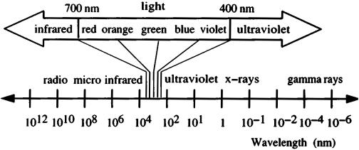
CHAPTER 2. RENDERING CONCEPTS 2.2 BASIC OPTICS

Figure 2.1: Electromagnetic spectrum.

2.2 Basic Optics

Light is a form of electromagnetic radiation, a sinusoidal wave formed by coupled electric and magnetic fields. The electric and magnetic fields are perpendicular to each other and to the direction of propagation. The frequency of the oscillation determines the wavelength. Electromagnetic radiation can exist at any wavelength. From long to short, there are radio waves, microwaves, infrared, light, ultraviolet, x-rays, and gamma rays (see Figure 2.1).

A pure source of light, such as that produced by a laser, consists of light at a single frequency. In the natural world, however, light almost always exists as a mixture of different wavelengths. Laser light is also coherent, that is, the source is tuned so that the wave stays in phase as it propagates. Natural light, in contrast, is incoherent.

Electromagnetic radiation can also be polarized. This refers to the preferential orientation of the electric and magnetic field vectors relative to the direction of propagation. Just as incoherent light consists of many waves that are summed with random phase, unpolarized light consists of many waves that are summed with random orientation. The polarization of the incident radiation is an important parameter affecting the reflection of light from a surface, but the discussion will be simplified by ignoring polarization.

The fact that light is just one form of electromagnetic radiation is of great benefit for computer graphics in that it points to theory and algorithms from many other disciplines, in particular, optics, but also more applied disciplines such as radar engineering and radiative heat transfer. The study of optics is typically divided into three subareas: geometrical or ray optics, physical or wave optics, and quantum or photon optics. Geometrical optics is most relevant to computer graphics since it focuses on calculating macroscopic properties of light

Radiosity and Realistic Image Synthesis	14
Edited by Michael F. Cohen and John R. Wallace

CHAPTER 2. RENDERING CONCEPTS

2.3 RADIOMETRY AND PHOTOMETRY

as it propagates through environments. Geometrical optics is useful to understand shadows, basic optical laws such as the laws of reflection and refraction, and the design of classical optical systems such as binoculars and eyeglasses. However, geometrical optics is not a complete theory of light. Physical or wave optics is necessary to understand the interaction of light with objects that have sizes comparable to the wavelength of the light. Physical optics allows us to understand the physics behind interference, dispersion, and technologies such as holograms. Finally, to explain in full detail the interaction of light with atoms and molecules quantum mechanics must be used. In the quantum mechanical model light is assumed to consist of particles, or photons. For the purposes of this book, geometrical optics will provide a full-enough view of the phenomena simulated with the radiosity methods.

2.3 Radiometry and Photometry

Radiometry is the science of the physical measurement of electromagnetic energy. Since all forms of energy in principle can be interconverted, a radiometric measurement is expressed in the SI units for energy or power, joules and watts, respectively. The amount of light at each wavelength can be measured with a spectroradiometer, and the resulting plot of the measurements is the spectrum of the source.

Photometry, on the other hand, is the psychophysical measurement of the visual sensation produced by the electromagnetic spectrum. Our eyes are only sensitive to the electromagnetic spectrum between the ultraviolet (380 nm) and the infrared (770 nm). The most prominent difference between two sources of light with different mixtures of wavelengths is that they appear to have different colors. However, an equally important feature is that different mixtures of light also can have different luminosities, or brightnesses.

Pierre Bouguer established the field of photometry in 1760 by asking a human observer to compare different light sources [35]. By comparing an unknown source with a standard source of known brightness—a candle at the time—the relative brightness of the two sources could be assessed. Bouguer’s experiment was quite ingenious. He realized that a human observer could not provide an accurate quantitative description of how much brighter one source was than another, but could reliably tell whether two sources were equally bright.1 Bouguer was also aware of the inverse square law. Just as Kepler and Newton had used it to describe the gravitational force from a point mass source, Bouguer reasoned that it also applied to a point light source. The experiment consisted of the

1This fact will be used in Chapter 9 when algorithms to select pixel values for display are examined.

Radiosity and Realistic Image Synthesis	15
Edited by Michael F. Cohen and John R. Wallace

CHAPTER 2. RENDERING CONCEPTS

2.3 RADIOMETRY AND PHOTOMETRY

Figure 2.2: Spectral luminous relative efficiency curve.

observer moving the standard source until the brightnesses of the two sources were equal. By recording the relative distances of the two light sources from the eye, the relative brightnesses can be determined with the inverse square law.

Bouguer founded the field of photometry well before the mechanisms of human vision were understood. It is now known that different spectra have different brightnesses because the pigments in our photoreceptors have different sensitivities or responses toward different wavelengths. A plot of the relative sensitivity of the eye across the visible spectrum is shown in Figure 2.2; this curve is called the spectral luminous relative efficiency curve. The observer’s response, R, to a spectrum is then the sum, or integral, of the response to each spectral band. This in turn is equal to the amount of energy at that wavelength, l, times its relative luminosity.

R = ò770 V(λ )S(λ )dλ (2.1)

380 nm

where V is the relative efficiency and S is the spectral energy. Because there is wide variation between people’s responses to different light sources, V has been standardized.

Radiometry is more fundamental than photometry, in that photometric quantities may be computed from spectroradiometric measurements. For this reason, it is best to use radiometric quantities for computer graphics and image synthesis. However, photometry preceded radiometry by over a hundred years, so much of radiometry is merely a modern interpretation of ideas from photometry.

As mentioned, the radiometric units for power and energy are the watt and joule, respectively. The photometric unit for luminous power is the lumen, and the photometric unit for luminous energy is the talbot. Our eye is most

Radiosity and Realistic Image Synthesis	16
Edited by Michael F. Cohen and John R. Wallace

CHAPTER 2. RENDERING CONCEPTS 2.4 THE LIGHT FIELD

sensitive to yellow-green light with a wavelength of approximately 555 nm that has a luminosity of 684 lumens per watt. Light of any other wavelength, and therefore any mixture of light, will yield fewer lumens per watt. The number of lumens per watt is a rough measure of the effective brightness of a light source. For example, the garden-variety 40-Watt incandescent light bulb is rated at only 490 lumens—roughly 12 lumens per watt. Of course, the wattage in this case is not the energy of the light produced, but rather the electrical energy consumed by the light bulb. It is not possible to convert electrical energy to radiant energy with 100% efficiency so some energy is lost to heat.

When we talk about light, power and energy usually may be used interchangeably, because the speed of light is so fast that it immediately attains equilibrium. Imagine turning on a light switch. The environment immediately switches from a steady state involving no light to a state in which it is bathed in light. There are situations, however, where energy must be used instead of power. For example, the response of a piece of film is proportional to the total energy received. The integral over time of power is called the exposure. The concept of exposure is familiar to anyone who has stayed in the sun too long and gotten a sunburn.

An important principle that must be obeyed by any physical system is the conservation of energy. This applies at two levels—a macro or global level, and a micro or local level.

•At the global level, the total power put into the system by the light sources must equal the power being absorbed by the surfaces. In this situation energy is being conserved. However, electrical energy is continuing to flow into the system to power the lights, and heat energy is flowing out of the system because the surfaces are heated.

•At the local level, the energy flowing into a region of space or onto a surface element must equal the energy flowing out. Accounting for all changes in the flow of light locally requires that energy is conserved. Thus, the amount of absorbed, reflected, and transmitted light must never be greater than the amount of incident light. The distribution of light can also become more concentrated or focused as it propagates. This leads to the next topic which is how to characterize the flow of light.

2.4The Light Field

2.4.1 Transport Theory

The propagation of light in an environment is built around a core of basic ideas concerning the geometry of flows. In physics the study of how “stuff” flows

Radiosity and Realistic Image Synthesis	17
Edited by Michael F. Cohen and John R. Wallace

CHAPTER 2. RENDERING CONCEPTS 2.4 THE LIGHT FIELD

Figure 2.3: Particles in a differential volume.

is termed transport theory. The “stuff” can be mass, charge, energy, or light. Flow quantities are differential quantities that can be difficult to appreciate and manipulate comfortably. In this section all the important physical quantities associated with the flow of light in the environment will be introduced along with their application to computer graphics.

The easiest way to learn transport quantities is to think in terms of particles (think of photons). Particles are easy to visualize, easy to count, and therefore easy to track as they flow around the environment. The particle density p(x) is the number of particles per unit volume at the point x (see Figure 2.3). Then the total number of particles, P(x), in a small differential volume dV is

P(x) = p(x) dV

(2.2)

Note that the particle density is an intrinsic or differential quantity, whereas the total number of particles is an absolute or extrinsic quantity.

Now imagine a stream of particles all moving with the same velocity vector v ; that is, if they are photons, not only are they all moving at the speed of light, but they are all moving in the same direction. We wish to count the total number of particles flowing across a small differential surface element dA in a slice of time dt. The surface element is purely fictitious and introduced for convenience and may or may not correspond to a real physical surface. In time dt each particle moves a distance v dt. How many particles cross dA? This can be computed using the following observation: consider the tube formed by sweeping dA a distance vdt in the direction –v . All particles that cross dA between t and t + dt must have initially been inside this tube at time t. If they were outside this tube, they would not be moving fast enough to make it to the surface element dA in the allotted time. This implies that one can compute the number of particles crossing the surface element by multiplying the particle volume density times the volume of the tube. The volume of the tube is just equal to its base (dA) times its height, which is equal to v cos θ dt. Therefore, as depicted in Figure 2.4, the total number of particles crossing the surface is

P(x) = p(x) dV
= p(x)(v dt cos θ) dA	(2.3)
Radiosity and Realistic Image Synthesis	18
Edited by Michael F. Cohen and John R. Wallace