Cohen M.F., Wallace J.R. - Radiosity and realistic image synthesis (1995)(en)

CHAPTER 2. RENDERING CONCEPTS 2.4. THE LIGHT FIELD

Figure 2.4: Total particles crossing a surface.

Note that the number of particles flowing through a surface element depends on both the area of the surface element and its orientation relative to the flow. Observe that the maximum flow through a surface of a fixed size occurs when the surface is oriented perpendicular to the direction of flow. Conversely, no particles flow across a surface when it is oriented parallel to the flow. More specifically, the above formula says that the flow across a surface depends on the cosine of the angle of incidence between the surface normal and the direction of the flow. This fact follows strictly from the geometry of the situation and does not depend on what is flowing.

The number of particles flowing is proportional both to the differential area of the surface element and to the interval of time used to tally the particle count. If either the area or the time interval is zero, the number of particles flowing is also zero and not of much interest. However, we can divide through by the time interval dt and the surface area dA and take the limit as these quantities go to zero. This quantity is called the flux.

More generally all the particles through a point will not be flowing with the same speed and in the same direction. Fortunately, the above calculation is fairly easy to generalize to account for a distribution of particles with different velocities moving in different directions. The particle density is now a function of two independent variables, position x and direction ω . Then, just as before, the

number of particles flowing across a differential surface element in the direction
ω equals	ω ) = p(x, ω ) cos θ dω dA
P(x,		(2.4)

Here the notation dω is introduced for the differential solid angle. The direction of this vector is in the direction of the flow, and its length is equal to the small differential solid angle of directions about ω . For those unfamiliar with solid angles and differential solid angles, please refer to the box.

2.4.2 Radiance and Luminance

The above theory can be immediately applied to light transport by considering ight as photons. However, rendering systems almost never need consider (or at

Radiosity and Realistic Image Synthesis	19
Edited by Michael F. Cohen and John R. Wallace

CHAPTER 2. RENDERING CONCEPTS 2.4 THE LIGHT FIELD

Angles and Solid Angles

A direction is indicated by the vector . Since this is a unit vector, it can be represented by a point on the unit sphere. Positions on a sphere in turn can be represented by two angles: the number of degrees from the North Pole or zenith, θ, and the number of degrees about the equator or azimuth, φ. Directions ω and spherical coordinates (θ, φ) can be used interchangeably.

A big advantage of thinking of directions as points on a sphere comes when considering differential distributions of directions. A differential distribution of directions can be represented by a small region on the unit sphere.

least have not considered up to this point) the quantum nature of light. Instead, when discussing light transport, the stuff that flows, or flux, is the radiant energy per unit time, or radiant power Φ, rather than the number of particles. The radiant energy per unit volume is simply the photon volume density times the energy of a single photon h c/λ, where h is Planck’s constant and c is the speed of light. The radiometric term for this quantity is radiance.

L(x, ω ) = ò	p(x, ω , λ)	hc
			dλ	(2.6)
		λ

Radiance is arguably the most important quantity in image synthesis. Defined precisely, radiance is power per unit projected area perpendicular to the ray per unit solid angle in the direction of the ray (see Figure 2.5). The definition in equation 2.6 is that proposed by Nicodemus [174], who was one of the first authors to recognize its fundamental nature.

The radiance distribution completely characterizes the distribution of light

Radiosity and Realistic Image Synthesis	20
Edited by Michael F. Cohen and John R. Wallace

CHAPTER 2. RENDERING CONCEPTS 2.4. THE LIGHT FIELD

The area of a small differential surface element on a sphere of radius r is

dA = (r dθ) (r sin φ dφ) = r2 sin θ dθ dφ

Here rdθ is the length of the longitudinal are generated as θ goes to θ + dθ. Similarly r sin θdφ is the length of the latitudinal are generated as φ goes to φ + dφ. The product of these two lengths is the differential area of that patch on the sphere.

This derivation uses the definition of angle in radians: the angle subtended by a circular arc of length l is equal to l/r. The circle itself subtends an angle of 2π radians because the circumference of the circle is 2πr. By using a similar idea we can define a solid angle. The solid angle subtended by a spherical area a is equal to a/r2. This quantity is the measure of the angle in steradians (radians squared), denoted sr. A sphere has a total area of 4πr2, so there are 4π steradians in a sphere.

A differential solid angle, indicated as dω, is then

dA

dω = = sin θ dθ dφ (2.5)

r2

It is very convenient to think of the differential solid angle as a vector, d ω . The direction of d ω is in the direction of the point on the sphere, and the length of d ω is equal to the size of the differential solid angle in that direction.

Figure 2.5: The radiance is the power per unit projected area perpendicular to the ray per unit solid angle in the direction of the ray.

Radiosity and Realistic Image Synthesis	21
Edited by Michael F. Cohen and John R. Wallace

CHAPTER 2. RENDERING CONCEPTS 2.4 THE LIGHT FIELD

Figure 2.6: Equality of flux leaving the first surface and flux arriving on the second surface.

in a scene. Note that it is a function of five independent variables, three that specify position and two that specify direction. All other radiometric quantities can be computed from it. For example, the differential flux in a small beam with cross-sectional area dA and differential solid angle dω is

dΦ = L(x, ω ) cos θ dω dA

(2.7)

This follows immediately from the earlier discussion of particle transport.

To emphasize further the importance of radiance, consider the following two properties:

l. The radiance in the direction of a light ray remains constant as it propagates along the ray (assuming there are no losses due to absorption or scattering). This law follows from the conservation of energy within a thin pencil of light, as shown in Figure 2.6.

The total flux leaving the first surface must equal the flux arriving on the second surface.

				L1		dω1 dA1 = L2 dω2 dA2		(2.8)
but dω	1	= dA	/r2	and dω	2	= dA	/r2, thus,
		2				1

	T = dω1 dA1 = dω2 dA2	=	dA1	dA2	(2.9)
			r2
	Radiosity and Realistic Image Synthesis				22
	Edited by Michael F. Cohen and John R. Wallace

CHAPTER 2. RENDERING CONCEPTS 2.4. THE LIGHT FIELD

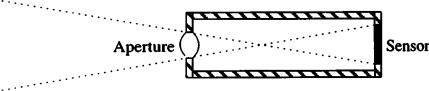
Figure 2.7: A simple exposure meter.

This quantity T is called the throughput of the beam; the larger the throughput, the bigger the beam. This immediately leads to the conclusion that

L1 = L2

(2.10)

and hence, the invariance of radiance along the direction of propagation.

As a consequence of this law, radiance is the numeric quantity that should be associated with a ray in a ray tracer.

2. The response of a sensor is proportional to the radiance of the surface visible to the sensor.

To prove this law, consider the simple exposure meter in Figure 2.7. This meter has a small sensor with area a and an aperture with area A. The response of the sensor is proportional to the total integrated flux falling on it.

R = òA òΩ L cos θ dω dA = LT

(2.11)

Thus, assuming the radiance is constant in the field of view, the response is proportional to the radiance. The constant of proportionality is the throughput, which is only a function of the geometry of the sensor. The fact that the radiance at the sensor is the same as the radiance at the surface follows from the invariance of radiance along a ray.

This law has a fairly intuitive explanation. Each sensor element sees that part of the environment inside the beam defined by the aperture and the receptive area of the sensor. If a surface is far away from the sensor, the sensor sees more of it. Paradoxically, one might conclude that the surface appears brighter because more energy arrives on the sensor. However, the sensor is also far from the surface, which means that the sensor subtends a smaller angle with respect to the surface. The increase in energy resulting from integrating over a larger surface area is exactly counterbalanced by the decrease in percentage of light that makes it to the sensor. This property of radiance explains why a large uniformly illuminated painted wall appears equally bright over a wide range of viewing distances.

Radiosity and Realistic Image Synthesis	23
Edited by Michael F. Cohen and John R. Wallace

CHAPTER 2. RENDERING CONCEPTS 2.4 THE LIGHT FIELD

Figure 2.8: Projection of differential area.

As a consequence, the radiance from a surface to the eye is the quantity that should be output to the display device.

2.4.3 Irradiance and Illuminance

The two properties of radiance described in the previous section were derived by considering the total flux within a small beam of radiation. Another very important quantity is the total energy per unit area incident onto a surface with a fixed orientation. This can be computed by integrating the incident, or incoming radiance, Li , over a hemisphere, Ω.

dΦ =	é	L cos θ dω ù		dΑ	(2.12)
	ê	i	ú
	ëòΩ		û

The irradiance, E, is the radiant energy per unit area falling on a surface (the corresponding photometric quantity is the illuminance).

	Ε º	dF		(2.13)
		dΑ
or	òΩL cos θ dω
Ε =				(2.14)

The quantity cos θ dw is often referred to as the projected solid angle. It can be thought of as the projection of a differential area on a sphere onto the base of the sphere, as shown in Figure 2.8.

This geometric construction shows that the integral of the projected solid angle over the hemisphere is just π, the area of the base of a hemisphere with

Radiosity and Realistic Image Synthesis	24
Edited by Michael F. Cohen and John R. Wallace

CHAPTER 2. RENDERING CONCEPTS 2.4. THE LIGHT FIELD

unit radius. This result can also be derived directly by computing the following integral:

	2 π		π
òΩcos θ dω = ò0		ò0 cos				θ sin θ dθ dφ
		2 π			π
=	– ò0				ò0 cos θ d cos θ dφ
=	–2π			cos2		θ			π / 2
					2				0
= π
						(2.15)

Note that if all rays of light are parallel, which occurs if a single distant source irradiates a surface, then the integral reduces to the simple formula

E = E0 cos θ

(2.16)

where E0 is the energy per unit perpendicular area arriving from the distant source.

2.4.4 Radiosity and Luminosity

As the title of this book suggests, radiosity is another important quantity in image synthesis. Radiosity, B, is very similar to irradiance. Whereas irradiance is the energy per unit area incident onto a surface, radiosity is the energy per unit area that leaves a surface. It equals

B = òΩ Lo cos θ dω

(2.17)

where Lo is the outgoing radiance.

The official term for radiosity is radiant exitance. Because of the widespread use of the term radiosity in the computer graphics literature, it will be used in this book. The photometric equivalent is luminosity.

2.4.5 Radiant and Luminous Intensity

Radiance is a very useful way of characterizing light transport between surface elements. Unfortunately, it is difficult to describe the energy distribution of a point light source with radiance because of the point singularity at the source. Fortunately, it is very easy to characterize the energy distribution by introducing another quantity—the radiant or luminous intensity.

Radiosity and Realistic Image Synthesis	25
Edited by Michael F. Cohen and John R. Wallace

CHAPTER 2. RENDERING CONCEPTS 2.4 THE LIGHT FIELD

Note that this use of “intensity” is very different from that typically used by the computer graphics community. Even more confusion results because intensity is often used to indicate radiance-like transport quantities in the physics community. The radiant intensity is quite similar to that used in the geometric optics community.

The energy distribution from a point light source expands outward from the center. A small beam is defined by a differential solid angle in a given direction. The flux in a small beam dw is defined to be equal to

dΦ ≡ I ( ω ) dω

(2.18)

I is the radiant intensity of the point light source with units of power per unit solid angle. The equivalent photometric quantity is the luminous intensity.

The radiant intensity in a given direction is equal to the irradiance at a point on the unit sphere centered at the source. In the geometric optics literature intensity is defined to be the power per unit area (rather than per unit solid angle). In the case of a spherical wavefront emanating from a point source, the geometric optics definition is basically the same as the radiometric definition. However, in general, the wavefront emanating from a point source will be distorted after it reflects or refracts from other surfaces and so the definition in terms of solid angle, is less general.

For an isotropic point light source,

	I =	Φ	(2.19)
		4π

Of course, a point source may act like a spotlight and radiate different amounts of light in different directions. The total energy emitted is then

Φ = òΩ I ( ω ) dω

(2.20)

The irradiance on a differential surface due to a single point light source can be computed by calculating the solid angle subtended by the surface element from the point of view of the light source.

E = I	dω	=	Φ cos θ					(2.21)
	dΑ		4π		x – xS		2

where x – xS is the distance from the point to the surface element. Note the 1/r2 fall-off: this is the origin of the inverse square law.

The distribution of irradiance on a surface is often drawn using a contour plot or iso-lux diagram, while the directional distribution of the intensity from a point light source is expressed with a goniometric or iso-candela diagram.2 This is a contour plot of equal candela levels as a function of the (θ,φ).

2See Chapter 10 for details of lighting specifications.

Radiosity and Realistic Image Synthesis	26
Edited by Michael F. Cohen and John R. Wallace

CHAPTER 2. RENDERING CONCEPTS 2.4. THE LIGHT FIELD

Physics	Radiometry	Radiometric Units
	Radiant energy	joules [J = kgm2/s2]
Flux	Radient power	watss [W = joules/s]
Angular flux density	Radiance	[W/m2sr]
Flux density	Irradiance	[W/m2]
Flux density	Radiosity	[W/m2]
	Radiant intensity	[W/sr]

Physics	Photometry	Photometric Units
	Luminous energy	talbot
Flux	Luminous power	lumens [talbot/second]
Angular flux density	Luminance	Nit [lumens/m2sr]
Flux density	Illuminance	Lux [lumens/m2sr]
Flux density	Luminosity	Lux [lumens/m2sr]
	Luminous intensity	Candela [lumens/sr]

Table 2.1: Radiometric and photometric quantities.

2.4.6 Summary of Radiometric and Photometric Quantities

In most computer graphics systems, optical quantities are simply colors denoted by red, green, and blue triplets. These triplets are used to specify many quantities including light sources, material properties, and intermediate calculations.3 As noted, there is a small but finite number (six to be exact) of radiometric (photometric) quantities that characterize the distribution of light in the environment. They are the radiant energy (luminous energy), radiant power (luminous power), radiance (luminance), irradiance (illuminance), radiosity (luminosity), and radiant intensity (luminous intensity). These quantities and their units are summarized in Table 2.1.

3A more complete treatment of color specification is given in Chapter 9.

Radiosity and Realistic Image Synthesis	27
Edited by Michael F. Cohen and John R. Wallace

CHAPTER 2. RENDERING CONCEPTS 2.5. REFLECTION FUNCTIONS

Figure 2.9: Bidirectional reflection distribution function.

2.5 Reflection Functions

The next question is how to characterize the reflection of light from a surface. Reflection is defined as the process by which light incident on a surface leaves that surface from the same side. Transmission, absorption, spectral and polarization effects, fluorescence, and phosphorescence are also important to consider in developing an accurate model of the interaction of light with materials, but will not be treated in detail here. Instead, this section will concentrate on nomenclature and the general properties that are satisfied by all reflection functions.

2.5.1 The Bidirectional Reflection Distribution Function

Consider the light incident on a surface from a small differential solid angle in the direction ω i. The amount of reflected light in another direction ω r is proportional to the incident irradiance from ω i (see Figure 2.9). That is,

dLr ( ω r ) dE ( ω i )

(2.22)

Equation 2.22 simply states that an increase in the incident light energy per unit area results in a corresponding increase in the reflected light energy. The incident irradiance can be increased by increasing either the solid angle subtended by the source or the energy density in the beam.

The constant of proportionality is termed the bidirectional reflection distribution function, or BRDF.

f r (ωi → ωr ) ≡	Lr	(ωr )
			(2.23)
	Li (ωi ) cos θi dωi
Radiosity and Realistic Image Synthesis		28
Edited by Michael F. Cohen and John R. Wallace