32 4 Word-Length Optimization

word-length nj2 > nj1 + n, then this assignment is sub-optimal, since at most nj1 + n bits are necessary to represent the result to full precision. Ensuring that such cases do not arise is referred to as ‘conditioning’ the annotated computation graph [CCL01b]. Conditioning is an important design step, as it allows the search space of e cient implementations to be pruned, and ensures that the most e cient use is made of all bits of each signal. It is now possible to define a well-conditioned annotated computation graph to be one in which there are no superfluous bits representing any signal (Definition 4.2).

Definition 4.2. An annotated computation graph G (V, S, A) with A = (n, p) is said to be well-conditioned i nj ≤ nqj for all j S.

During word-length optimization, ill-conditioned graphs may occur as intermediate structures. An ill-conditioned graph can always be transformed into an equivalent well-conditioned form in the iterative manner shown in Algorithm WLCondition.

Algorithm 4.1 Algorithm WLCondition

Input: An annotated computation graph G (V, S, A)

Output: An annotated computation graph, with well-conditioned word-lengths and identical behaviour to the input system

begin

Calculate pj and nqj for all signals j S (Table 4.1)

Form nqj from nqj , pj and pj for all signals j S while j S : nqj < nj

Set nj ← nqj

Update nqj for all a ected signals (Table 4.1) Re-form nqj from nqj , pj and pj for all a ected signals

end while end

4.1.2 Linear Time-Invariant Systems

We shall first address error estimation for linear time-invariant systems. An appropriate noise model for truncation of least-significant bits is introduced below. It is shown that the noise injected through truncation can be analytically propagated through the system, in order to measure the e ect of such a noise on the system outputs. Finally, the approach is extended in order to provide detailed spectral information on the noise at system outputs, rather than simply a signal-to-noise ratio.

Noise Model

A common assumption in DSP design is that signal quantization (rounding or truncation) occurs only after a multiplication or multiply-accumulate operation. This corresponds to a uniprocessor viewpoint, where the result of

121 2

4.1 Error Estimation

33

an n-bit signal multiplied by an n-bit coe cient needs to be stored in an n-bit register. The result of such a multiplication is a 2n-bit word, which must therefore be quantized down to n bits. Considering signal truncation, the least area-expensive method of quantization [Fio98], the lowest value of the truncation error in two’s complement with p = 0 is 2−2n − 2−n ≈ −2−n and the highest value is 0. It has been observed that values between these ranges tend to be equally likely to occur in practice, so long as the 2n-bit signal has su cient dynamic range [Liu71, OW72]. This observation leads to the formulation of a uniform distribution model for the noise [OW72], of variance σ2 = −2n for the standard normalization of p = 0. It has also been observed that, under the same conditions, the spectrum of such errors tends to be white, since there is little correlation between low-order bits over time even if there is a correlation between high-order bits. Similarly, di erent truncations occurring at di erent points within the implementation structure tend to be uncorrelated.

When considering a multiple word-length implementation, or alternative truncation locations, some researchers have opted to carry this model over to the new implementation style [KS98]. However there are associated inaccuracies involved in such an approach [CCL99]. Firstly quantizations from n1 bits to n2 bits, where n1 ≈ n2, will su er in accuracy due to the discretization of the error probability density function. Secondly in such cases the lower bound on error can no longer be simplified in the preceding manner, since 2−n2 − 2−n1 ≈ −2−n1 no longer holds. Thirdly the multiple outputs from a branching node may be quantized to di erent word-lengths; a straight forward application of the model of [OW72] would not account for the correlations between such quantizations. Although these correlations would not a ect the probability density function, they would cause inaccuracies when propagating these error signals through to primary system outputs, in the manner described below.

The first two of these issues may be solved by considering a discrete probability distribution for the injected error signal. For two’s complement arith-

metic the truncation error injection signal e[t] caused by	truncation from
(n1, p) to (n2, p) is bounded by (4.1).
−2p(2−n2 − 2−n1 ) ≤ e[t] ≤ 0	(4.1)

It is assumed that each possible value of e[t] has equal probability, as discussed above. For two’s complement truncation, there is non-zero mean E{e[t]} (4.2) and variance σe2 (4.3).

		1		2n1−n2 −1
E{e[t]} = −					i · 2p−n1	(4.2)
			2n1−n2	=0
=	−	2p−1(2−n2i			2−n1 )
				−

34

4 Word-Length Optimization

n1−n2

−

1

σ2 =

1

2

(i 2p−n1 )2

E2 e[t]

n n

=

12

22p(2−2 2

− 2−

·

1 )

− { }

(4.3)

e

2

1−

2

i=0

1

n

2n

Note that for n1 n2 and p = 0, (4.3) simplifies to σe2 ≈ 121 2−2n2 which is the well-known predicted error variance of [OS75] for a model with continuous probability density function and n1 n2.

A comparison between the error variance model in (4.3) and the standard model of [OS75] is illustrated in Fig. 4.4(a), showing errors of tens of percent can be obtained by using the standard simplifying assumptions. Shown in Fig. 4.4(b) is the equivalent plot obtained for a continuous uniform distribution in the range [2−n1 − 2−n2 , 0] rather than [2−n2 , 0], which shows even further increases in error. It is clear that the discretization of the distribution around n1 ≈ n2 may have a very significant e ect on σe2. While in a uniform word-length implementation this error may not be large enough to impact on the choice of word-length, multiple word-length systems are much more sensitive to such errors since finer adjustment of output signal quality is possible.

error (%)

0.35

0.3

0.25

0.2

0.1
0.05	15
0	10
16
0.15

14
12		5
10			n2
8	6
n1	4
	2	0
	0

error (%)

0
−0.1
−0.2
−0.3
−0.4
−0.5
−0.6
−0.7	15
20

15		10
	10	5
n1	5	n2
	0	0

(a) (b)

Fig. 4.4. Error surface for (a) Uniform [2−n2 , 0] and (b) Uniform [2−n1 − 2−n2 , 0]

Accuracy is not the only advantage of the proposed discrete model. Consider two chained quantizers, one from (n0, p) to (n1, p), followed by one from (n1, p) bits to (n2, p) bits, as shown explicitly in Fig. 4.5. Using the error model of (4.3), the overall error variance injected, assuming zero correlation,

is σe20 + σe21 = 121 22p(2−2n1 − 2−2n0 + 2−2n2 − 2−2n1 ). This quantity is equal to σe22 = 121 22p(2−2n2 − 2−2n0 ). Therefore the error variance injected by considering a chain of quantizers is equal to that obtained when modelling the

chain as a single quantizer. This is not the case with either of the continuous uniform distribution models discussed. The standard model of [OW72] gives

σe20 + σe21 = 121 (22(p−n1) + 22(p−n2)). This is not equal to σe22 = 121 22(p−n2), and diverges significantly for n2 ≈ n1. This consistency is another useful advantage

of the proposed truncation model.

(n0,p)

(n0,p)

Q

+

(n1,p)

(n1,p)

Q

+

	4.1	Error Estimation			35
(n 2,p)	(n0,p)			(n2,p)
			Q
(n 2,p)	(n0,p)			(n2,p)

+

e 0[t]	e 1[t]	e 2[t]
(a) Two chained quantizers		(a) An equivalent structure

Fig. 4.5. (a) Two chained quantizers and their linearized model and (b) an equivalent structure and its linearized model

Noise Propagation and Power Estimation

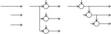
Given an annotated computation graph G (V, S, A), it is possible to use the truncation model described in the previous section to predict the variance of each injection input. For each signal j {(v1, v2) S : type(v1) =fork} a straight-forward application of (4.3) may be used with n1 = nqj , n2 = nj , and p = pj , where nqj is as defined in Section 4.1.1. Signals emanating from nodes of fork type must be considered somewhat di erently. Fig. 4.6(a) shows one such annotated fork structure, together with possible noise models in Figs. 4.6(b) and (c). Either model is valid, however Fig. 4.6(c) has the advantage that the error signals e0[t], e1[t] and e2[t] show very little correlation in practice compared to the structure of Fig. 4.6(b). This is due to the overlap in the low-order bits truncated in Fig. 4.6(b). Therefore the cascaded model is preferred, in order to maintain the uncorrelated assumption used to propagate these injected errors to the primary system outputs. Note also that the transfer function from each injection input is di erent under the two models. If in Fig. 4.6(b) the transfer functions from injection error inputs e0[t], e1[t] and e2[t] to a primary output k are given by t0k (z), t1k (z) and t2k (z), respectively, then for the model of Fig. 4.6(c), the corresponding transfer functions are t0k (z) + t1k (z) + t2k (z), t1k (z) + t2k (z) and t2k (z).

By constructing noise sources in this manner for an entire annotated computation graph G (V, S, A), a set F = {(σp2, Rp)} of injection input variances σp2, and their associated transfer function to each primary output Rp(z), can be constructed. From this set it is possible to predict the nature of the noise appearing at the system primary outputs, which is the quality metric of importance to the user. Since the noise sources have a white spectrum and are uncorrelated with each other, it is possible to use L2 scaling to predict the noise power at the system outputs. The L2-norm of a transfer function H(z) is defined in Definition 4.3. It can be shown that the noise variance Ek at output k is given by (4.4).

36	4 Word-Length Optimization
						e 0[t]				e 0[t]
	(9,0)	(8,0)		(9,0)		(8,0)			(9,0)	(8,0)
	3		0	3	+	0			3	+		0
			(7,0)			e 1[t]			e [t]		(7,0)
									1	+
			1		+	(7,0)						1
						1						(6,0)
			(6,0)
						e 2[t]				e 2[t]	+
												2
		2
						(6,0)
					+
						2
	(a) a FORK			(b) injection inputs					(c) cascaded injection
	node
				at each output						inputs
				Fig. 4.6. Modelling post-fork truncation
				Ek =	(σp , p			σp2L22{Rpk }				(4.4)
						R )		F

Definition 4.3. The L2-norm [Jac70] of a transfer function H(z) is given by (4.5), where Z−1{·} denotes the inverse z-transform.

L2{H(z)} = 2π π		1
		|H(ejθ )|2dθ
	π	2
1	−
		1	(4.5)
∞		2

=|Z−1{H(z)}[n]|2

n=0

Noise Spectral Bounds

There are some circumstances in which the SNR is not a su cient quality metric. One such circumstance is if the user is especially concerned about noise in particular frequency bands. Consider, for example, the four output noise spectra illustrated in Fig. 4.7. All spectra have identical power, however environments sensitive to noise at roughly half the Nyquist frequency are unlikely to favour the top-left spectrum. Similarly environments sensitive to high-frequency or low-frequency noise are unlikely to favour the bottomleft or top-right spectra, respectively. Under these circumstances it is useful to explore fixed-point architectures having error spectra bounded by a user specified spectrum function. The two approaches of noise power and noise spectrum bounds complement each other, and may be used either together or separately to guide the word-length optimization procedures to be discussed in this chapter.

This can be achieved by predicting the entire power spectral density (PSD). The noise PSD Qk(z) at an output k V of the algorithm may

4.1 Error Estimation

37

	100
spectrum	10−5
Noise power	10−10
	10−15
	0	0.2	0.4	0.6	0.8	1
	100
power spectrum	10−5
	10−10
Noise
	10−15	0.2	0.4	0.6	0.8	1
	0
		Normalized frequency (Nyquist = 1)

100
10−5
10−10
10−15	0.2	0.4	0.6	0.8	1
0
101
100
10−1
10−2	0.2	0.4	0.6	0.8	1
0
	Normalized frequency (Nyquist = 1)

Fig. 4.7. Some di erent noise spectra with identical noise power

be estimated using the transfer functions Rpk (z) from each noise source to the output as in (4.6), since each noise source has a white spectrum.

Qk(z) =	p , p		σp2|Rpk (z)|2, (z = ejθ )	(4.6)
(σ	R ) F

Once the noise PSD of a candidate implementation G (V, S, A) has been predicted, it is necessary to test whether the implementation satisfies the userspecified constraints. The proposed procedure tests an upper-bound constraint |Ck (ejθ )|2 for Qk (z), defined for all θ [0, 2π) by a real and rational function Ck (z). The feasibility requirement can be expressed as (4.7).

Qk(ejθ ) < |Ck (ejθ )|2, for all θ [0, π]

(4.7)

If there is an output k such that Qk(ej0) ≥ |Ck (ej0)|2 or Qk(ejπ ) ≥ |Ck (ejπ )|2 then clearly (4.7) does not hold and the feasibility test is complete. If neither of these conditions are true, and neither Qk(z) nor Ck (z) have poles on the unit circle |z| = 1, then we may partition the set [0, π] into

2n + 1 subsets {Θ1 = [0, θ1), Θ2 = [θ1, θ2), . . . , Θ2n+1 = [θ2n, π]} such that Qk (ejθ ) < |Ck (ejθ )|2 for θ Θ1 Θ3 . . . Θ2n and Qk (ejθ ) ≥ |Ck (ejθ )|2 for

θ Θ2 Θ4 . . . Θ2n−1. Since Qk (z) and Ck (z) have no poles on the unit circle, it may be deduced that Qk(ejθ1 )−|Ck (ejθ1 )|2 = Qk (ejθ2 )−|Ck (ejθ2 )|2 = Qk (ejθ2n ) − |Ck (ejθ2n )|2 = 0, and indeed that Qk (ejθ ) − |Ck (ejθ )|2 = 0 θ =