4.6 Some Results

69

Signals 0,2,4−6,8,11,13

	101
Spectrum	100
Power
	10−1

0

0.2

0.4

0.6

0.8

1

Signals 3,7

	100
Spectrum	10−1
Power	10−2
	10−3	0.2	0.4	0.6	0.8	1
	0
			Normalized frequency

Signals 9,12

100
10−1
10−2
10−3	0.2	0.4	0.6	0.8	1
0

Signals 1,10,14−18

100
10−5
10−10	0.2	0.4	0.6	0.8	1
0
		Normalized frequency

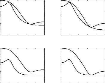
Fig. 4.24. Spectral profiles through the filter

area savings: for this example the uniform word-length design requires 810 logic cells in an Altera Flex10K device, compared to 636 and 663 logic cells for the shaped designs, a 22% and 18% area reduction respectively.

The spectral specifications are only slightly di erent in the two cases of Figs. 4.25(a) and (b): Fig. 4.25(b) has a somewhat reduced bound on highfrequency noise. The optimization procedure has successfully incorporated the modified constraint by reducing the high-frequency noise in the implemented structure. In contrast, there has been no change to the uniform word-length system between Figs. 4.25(c) and (d), since with a uniform word-length structure only a limited range of output noise spectra are possible.

4.6.2 Nonlinear Systems

Case Study: Adaptive Filtering

Adaptive filtering is a common DSP application, especially in the field of communications where it is widely used, for example, to compensate for multipath distortion in mobile communication systems [Hay96].

In addition to its practical significance, adaptive filtering has some interesting algorithmic features:

•All adaptive filtering algorithms contain feedback, limiting the applic-

ability of several existing word-length optimization techniques [WP98,

70 4 Word-Length Optimization

	10−4			(a)
Spectrum	10−5
Power	10−6
	10−7	0.2	0.4	0.6	0.8	1
	0
	10−4			(c)
Spectrum	10−5
Power	10−6
	10−7	0.2	0.4	0.6	0.8	1
	0
			Normalized frequency

10−4			(b)
10−5
10−6
10−7	0.2	0.4	0.6	0.8	1
0
10−4			(d)
10−5
10−6
10−7	0.2	0.4	0.6	0.8	1
0
		Normalized frequency

Fig. 4.25. Two specifications (upper curve) and their optimized (a,b) multiple word-length and (c,d) uniform word-length implementation noise spectra

NHCB01, BP00, SBA00, CRS+99] and limiting the performance achievable through pipelining.

•Adaptive filters contain general multipliers, rather than the constant coefficient multipliers present in static filters. This means that adaptive filters are nonlinear systems, limiting the applicability of purely analytic techniques such as that presented in Section 4.1.2 [CCL01b, CCL02].

•The coe cients of an adaptive filter are updated by accumulating (usually small) correction terms. Such ‘integration loops’ make the outputs of an adaptive filter very sensitive to errors induced around such loops.

The so-called least-mean-square (LMS) adaptive filter [Hay96] will be considered in this section, due to its widespread use in practice. For the unfamiliar reader, a brief review of LMS filters will now be provided.

Consider an input signal x[t] and a desired filter response d[t]. (The desired response could be known a-priori, for example from a ‘training sequence’ used in GSM mobile telephony). Let n denote the order of the filter, and u[t] denote the vector u[t] = (x[t] x[t − 1] x[t − 2] . . . x[t − n])T , where T represents vector/matrix transpose. An LMS filter with real input and coe cients has the following algorithm, where 0 represents a column vector with each element equal to 0, and µ is a user-chosen scalar adaptation coe cient.

4.6 Some Results

71

w[0] = 0 for t ≥ 0 do

y[t] = wT [t]u[t] e[t] = d[t] − y[t]

w[t + 1] = w[t] + µu[t]e[t] end do

A DFG for a first-order LMS filter is shown in Fig. 4.26. The DFG for an nth order filter is easily derived through a replication of the taps and the use of an adder-tree to sum the partial results.

x	F		z-1	F
	*	+ z-1 F *		* + z-1 F *
		+		F
		F	-1	+

y

d

filter taps

Fig. 4.26. First order LMS adaptive filter

Area, Power, and Speed

In order to demonstrate the area, power, and delay advantages of the proposed method, 90 filters of between 1st and 10th order have been constructed and synthesised. In each case the ‘desired’ input d[t] to the adaptive filter is a wellknown 100,000 sample voice clip from [FRE93]. The filter input x[t] is a version of the same signal, corrupted by three di erent 12th order autoregressive filters, operating on three disjoint and equally sized portions of the input signal. Each distortion filter has constant coe cients randomly chosen such that the filter poles occur in complex conjugate pairs and have independent, identically distributed uniform distribution in magnitude range (0, 1) and in phase range (0, π/2).

The filter designs and input sequences have then been passed to the synthesis tool, and for each design three di erent optimization procedures have been followed. Firstly, the design has been synthesized with the optimum uniform scaling and the optimum uniform word-length for all signals. This design choice reflects the simplest form of optimized DSP design. Secondly, the design has been synthesized with scaling individually optimized for each signal (see

72 4 Word-Length Optimization

Chapter 3) and the optimum uniform word-length. This design choice reflects the use of a tool such as [SBA00] which focuses on optimizing signals from the MSB-side. The final design procedure has been to use an individually optimized scaling combined with an individually optimized word-length, as proposed by this chapter.

From the filter designs in Simulink and the representative input sequences, the synthesis tool automatically generates a combination of structural VHDL and Xilinx Coregen scripts, together with a makefile to synthesize the Virtex bit-stream. Each design has been fully placed and routed in a Xilinx Virtex 1000 (XCV1000BG560-6), after which an area, power consumption, and timing analysis has been performed. Due to memory and run-time constraints imposed by large value-change-dump simulation files, power analysis could only be performed for a 100-sample portion of the 100,000-sample input sequence used by the tool.

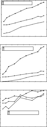
The first set of results is concerned with the variation of design metrics with the order of the filter to be synthesized. For each of these results, the filters have been synthesized using the same lower-bound on output SNR of 34dB.

The results are illustrated in Fig. 4.27(a), (b) and (c) for area, power, and clock period, respectively. Area savings of up to 37% (mean 32%) have been achieved over scaling optimization alone, and up to 63% (mean 61%) over neither scaling nor word-length optimization. This is combined with a power reduction of up to 49% (mean 43%) and speed-up of up to 18% (mean 10%) over scaling optimization alone, and a power reduction of up to 84.6% (mean 81.2%) and speed-up of up to 29% (mean 18%) over neither scaling nor word-length optimization.

The second set of results is concerned with the variation of design metrics with the user-specified lower-bound on allowable SNR. For these results, a 5th order LMS filter has been synthesized with SNR bound varying between −6dB and 64dB. These results are illustrated in Fig. 4.28(a), (b) and (c) for area, power, and clock period, respectively. As well as demonstrating the useful capability to trade-o numerical accuracy for area, power and speed, these results also illustrate significant improvements in all three metrics.

Area savings have been achieved of up to 75% (mean 45%) over scaling optimization alone, and up to 80% (mean 66%) over neither scaling nor wordlength optimization. This is combined with a power reduction of up to 96% (mean 58%) and speed-up of up to 29% (mean 11%) over scaling optimization alone, and a power reduction of up 98% (mean 87%) and speed up of up to 36% (mean 20%) over neither scaling nor word-length optimization.

It should be expected that on average the power savings are no smaller than the area savings of this approach. However in practice, the power savings are often significantly greater. This can be explained by two observations relating to the switching activity of signals. Firstly, if the scaling of each signal is not individually optimized, then a significant number of signals will contain unnecessary sign-extension. When a two’s complement signal changes from a

										4.6	Some Results	73
	4500
	4000		uniform scaling, uniform word−length
			optimized scaling, uniform word−length
			proposed method: optimized scaling, optimized word−length
	3500
	3000
(slices)	2500
area	2000
	1500
	1000
	500
	0	2	3	4	5	6	7	8	9	10
	1
					filter order

(a) variation of area with filter order

	180
	160		uniform scaling, uniform word−length
			optimized scaling, uniform word−length
	140		proposed method: optimized scaling, optimized word−length
	120
power (W)	100
	80
	60
	40
	20
	0	2	3	4	5	6	7	8	9	10
	1
					filter order

(b) variation of power consumption with filter order

80
70
60
50
(ns)		uniform scaling, uniform word−length
min40
		optimized scaling, uniform word−length
T
		proposed method: optimized scaling, optimized word−length
30
20
10
0	2	3	4	5	6	7	8	9	10
1
					filter order

(c) variation of minimum realizable clock period with filter order

Fig. 4.27. Synthesis results for LMS adaptive filters (fixed SNR bound of 34dB)

74 4 Word-Length Optimization

2500
	uniform scaling, uniform word−length
	optimized scaling, uniform word−length
	proposed method: optimized scaling, optimized word−length
2000
1500
area (slices)
1000
500
0	0	10	20	30	40	50	60	70
−10
			signal to quantization ratio (dBs)

(a) variation of area with SNR bound

	90
		uniform scaling, uniform word−length
	80	optimized scaling, uniform word−length
		proposed method: optimized scaling, optimized word−length
	70
	60
power (W)	50
	40
	30
	20
	10
	0	0	10	20	30	40	50	60	70
	−10
				signal to quantization ratio (dBs)

(b) variation of power consumption with SNR bound

	90
	80
	70
	60
(ns)	50
min
T	40
			uniform scaling, uniform word−length
			optimized scaling, uniform word−length
	30		proposed method: optimized scaling, optimized word−length
	20
	10
	0	0	10	20	30	40	50	60	70
	−10
				signal to quantization ratio (dBs)

(c) variation of minimum realizable clock period with SNR bound

Fig. 4.28. Synthesis results for LMS adaptive filters (5th order filter)