108 5 Saturation Arithmetic

		(a) uniform / sim
		(b) wl optimized / sim
	800	(d) comb optimized
		(e) uniform / l1
		(f) wl optimized / l1
	750
area
resulting system	700
	650
	600
	550	10−7
	10−8
		specified error variance

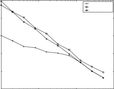
Fig. 5.17. Comparison of di erent design approaches for trading-o system area and error, for a 4th order lowpass elliptic IIR filter

strated that significant area reductions can be achieved for the narrow bandpass filter example. Fig. 5.18 illustrates how the area consumption of second order autoregressive filters varies with the location of their complex conjugate pole on the z-plane, for fixed error specification. Compared to 1 scaling, area savings have been achieved using the techniques developed in this chapter for systems with poles with magnitude greater than approximately 0.9.

5.6.2 Clock frequency results

As noted in Section 5.2, there are also significant timing overheads associated with the use of saturation arithmetic. While Algorithm CombOptAlg does not explicitly consider circuit speed, it is instructive to place the points on Fig. 5.16 on a speed / area design-space diagram. This is shown in Fig. 5.19, where the short simulation run results are used for representation of simulation-scaled systems. There are ten graphs, corresponding to the ten error variance specifications in Fig. 5.16. Speed estimates are obtained from Altera MaxPlus II [MAX] on the fully placed and routed design in an Altera Flex10kRC240-3 device. A Pareto-optimal point [DeM94] is a point in

5.6 Results and Discussion

109

450
			(a) comb optimized
			(b) uniform / l1
			(c) wl optimized / l1
400
350
area (#LCs)
300
250
200
10−3	10−2	10−1	100

distance of poles from |z|=1

Fig. 5.18. Variation of system area with pole location

the design space that is not dominated in all design objectives by any other design-space point. The Pareto optimal points in Fig. 5.19 are joined by solid lines.

The results of Fig. 5.19 demonstrate that although the di erence in area is small between short-run simulation-based scaling word-length-optimized systems and those resulting from Algorithm CombOptAlg, there is a significant speed di erence. The source of this consistent speedup, averaging 27.6% over uniform word-length and 23.7% over optimized word-length structures, is illustrated in Fig. 5.20 where the saturator locations and degrees are illustrated for a single optimization example.

Comparing Figs. 5.20(a) and (b), simulation-based scaling has resulted in a large number of low degree saturators. In contrast the optimized saturators are few in number, but are generally of higher degree. Although aiming to reduce system implementation area, Algorithm CombOptAlg has also resulted in significant speedup over simulation-based approaches by using only a small number of saturators. The Cauchy-Schwartz bound tends to drive the solution towards using fewer saturators in order to minimize the potential error crosscorrelation e ects.