98 5 Saturation Arithmetic

end

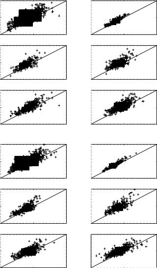
5.4.6 Error estimation results

This section presents some results from using the error model discussed thus far to predict saturation error variance. Approximately 6000 IIR filters have been generated, each filter having between second and tenth order. The feedback coe cients are generated by randomly choosing complex conjugate pole locations in the range 0 < |z| < 0.998 and 0 < arg(z) < π (uniformly distributed), and the feed-forward coe cients are generated by randomly distributing them between 0 and 1 (uniformly distributed). 1 scaling is then applied to each filter, and the binary point locations are decided by choosing either those through 1 scaling or one or two bits beneath this value, each location independently of the other. Probabilities are skewed such that there is a mean of two saturation nonlinearities in each section, in order to agree with typical synthesized circuits. The choice of saturator degree is decided with uniformly distributed probability and independently of all other saturation locations. The predicted error variance is then compared to the observed variance arrived at through a bit-true simulation of the system. Two types of input data are used: independent identically distributed Gaussian input samples, and real speech data [FRE93].

Fig. 5.13 presents several plots of the error bound, derived through the technique presented in this chapter, against a simulation run. Fig. 5.14 presents the data as a histogram of over-estimation ratios, and also illustrates how this histogram changes with the order of the filter modelled for the iid case. It is clear that for the large majority of designs the Cauchy-Schwartz bound provides a value between 0dB and 50dB greater than the simulated result. Although both the slackness of the bound derived, and the mismatch between the saturated Gaussian model and post-addition pdf grow with the order of the filter, it is not a rapid growth. From fourth to tenth order the bulk of overestimation ratios lie in the same range, with little change in the spread of the distribution. Recall that the error estimation is for average-case behaviour, and so the bound is on the expected error variance, not the error variance for each specific case. In addition the bound is only exact if the standard deviations of the injected errors are known exactly, whereas in reality they are estimated through modelling signals as saturated Gaussians, as discussed previously. There is some mismatch between the input probability density function and the Gaussian assumption for speech, leading to marginally worse performance in the speech case (speech pdf falls o as exp(−λ1|x|) rather than the Gaussian exp(−λ2x2) [P50]).

Whether the noise model is su cient for optimization purposes can only be measured by the quality of the circuits produced by the optimization procedure, which will be discussed in the following section.

5.4 Noise Model

99

bound	1010
	0
error	10
	10−10
	10−10
bound	1010
	0
error	10
	10−10
	10−10
bound	1010
	0
error	10
	10−10
	10−10
bound	1010
	0
	10
error
	10−10
	10−10
bound	1010
	0
error	10
	10−10
	10−10
bound	1010
	0
error	10
	10−10
	10−10

all filters (speech input)

100 1010 4th order filters

100 1010 8th order filters

100 1010 simulated error power

all filters (iid Gaussian input)

100 1010 4th order filters

100 1010 8th order filters

bound	1010
	0
error	10
	10−10
	10−10
bound	1010
	0
error	10
	10−10
	10−10
bound	1010
	0
error	10
	10−10
	10−10
bound	1010
	0
	10
error
	10−10
	10−10
bound	1010
	0
error	10
	10−10
	10−10
	1010

2nd order filters

100 1010 6th order filters

100 1010 10th order filters

100 1010 simulated error power

2nd order filters

100 1010 6th order filters

100 1010 10th order filters

	bound	0
		10
	error

		10−10
100	1010	10−10		100	1010
simulated error power				simulated error power

Fig. 5.13. Saturation error model: estimated against simulated error variance for (upper) speech input and (lower) iid Gaussian input

100 5 Saturation Arithmetic

bound−to−sim error ratio (dBs) for speech input

150
100
50
0	−100	−50	0	50	100	150
−150
		bound−to−sim error ratio (dBs) for iid Gaussian input
150
100
50
0	−100	−50	0	50	100	150
−150

2nd order filters

40
30
frequency
20
10
0
			−100	−50	0		50				100	150
−150
60				6th order filters
frequency 20
40

0	−100	−50	0	50	100	150
−150

10th order filters

80

60
frequency
40
20
0	−100	−50	0	50	100	150
−150
bound−to−sim error ratio (dB) for iid Gaussian

4th order filters

50

40

frequency 30 20

10
0	−100	−50	0	50	100	150
−150

8th order filters

80

60
frequency
40
20
0	−100	−50	0	50	100	150
−150
bound−to−sim error ratio (dB) for iid Gaussian

Fig. 5.14. Overestimation ratios for saturation error model (upper) over all filter orders and (lower) for specific filter orders