Ufimtsev P. Fundamentals of the physical theory of diffraction (Wiley 2007)(348s) PEo

72 Chapter 4 Radiation by the Nonuniform Component of Surface Sources

By summation with the incident wave (3.1), these equations determine the PO part of the total field:

us,h(0)t = us,h(0)d + us,hgo ,

(4.2)

where us,h(0)d is the diffracted part of the field, which is described by functions vs,h± . The geometrical optics part us,hgo of the PO field is the same quantity as that in Equation (4.1).

The field (4.1) is generated by total surface source js,h = js,h(0) + js,h(1), consisting of the uniform and nonuniform components, and the PO field (4.2) is radiated only by the uniform component js,h(0). Therefore, the field created by the nonuniform component is the difference

us,h(1) = us,ht − us,h(0)t = us,hd − us,h(0)d.

(4.3)

In the case 0 < ϕ0 < α − π , when only one face (ϕ = 0) is illuminated, this field is determined by

(1)	vs+(kr, ϕ, ϕ0),
us	/u0 = v(kr, ϕ − ϕ0) − v(kr, ϕ + ϕ0) − vs−(kr, ϕ, ϕ0),
and
(1)	vh+(kr, ϕ, ϕ0),
uh	/u0 = v(kr, ϕ − ϕ0) + v(kr, ϕ + ϕ0) − vh−(kr, ϕ, ϕ0),

with 0 ≤ ϕ < π with π < ϕ ≤ α,

(4.4)

with 0 ≤ ϕ < π with π < ϕ ≤ α.

(4.5)

In the case α − π < ϕ0 < π , when both faces are illuminated, the field us,h(1) is determined as

us(1)/u0 = v(kr, ϕ − ϕ0) − v(kr, ϕ + ϕ0)

−

s

+

s

−

−

−

−

v+(kr, ϕ, ϕ0)

v−(kr, α

ϕ, α

ϕ0),

ϕ < α

π

with 0

vs+(kr, ϕ, ϕ0)

+ vs+(kr, α

−

ϕ, α

−

ϕ0),

with α ≤

π < ϕ < π

(kr, ϕ, ϕ0)

v

(kr, α

ϕ, α

ϕ0),

with π < ϕ

α,

v

+

−

−

≤

s−

s+

(4.6)

uh(1)/u0 = v(kr, ϕ − ϕ0) + v(kr, ϕ + ϕ0)

−

−

−

v+(kr, ϕ, ϕ

)

+

v−(kr, α

−

ϕ, α

ϕ

),

ϕ < α

−

π

with 0

h

0

h

− ϕ, α

−

0

with α ≤

vh+(kr, ϕ, ϕ0)

+ vh+(kr, α

ϕ0),

π < ϕ < π

h

+ h

−

−

≤

v+(kr, α

ϕ, α

ϕ0),

with π < ϕ

α.

v−(kr, ϕ, ϕ0)

(4.7)

The function v(kr, ψ ) is defined in Equation (2.51) and the functions vs,h± (kr, ϕ, ϕ0) in Equations (3.39) and (3.40) by the integrals in the complex plane

TEAM LinG

4.1 Integrals and Asymptotics 73

over the same contour D0 shown in Figure 2.6. Therefore, the field us,h(1) can be represented as the integral over the contour D0 with the integrand consisting of a linear combination of the integrands related to functions v and vs,h± :

us,h(1) = D0	Us,h(α, ϕ, ϕ0, ζ )eikr cos ζ dζ .	(4.8)
For the observation points far away from the edge (kr		1), this integral can

be asymptotically evaluated by the saddle point method (Copson, 1965; Murray,

√

iπ/4

ζ

2e

sin

1984). To do this, we first replace the integration variable ζ by s =

2 and

transform the integral to the form

u(1)

√

2e−i π4 eikr ∞

Us,h[α, ϕ, ϕ0, ζ (s)]

e−krs2 ds.

(4.9)

s,h

=

−∞

cos

ζ (s)/2

]

[

We then expand the integrand Us,h/ cos(ζ /2) into the Taylor series in the vicinity of the saddle point s = 0, retain only the first term in this series, and obtain the asymptotic expression

(1)

π

∞

2

∞

2

us,h

= √2e−i 4 eikr Us,h(α, ϕ, ϕ0, 0)

−∞ e−krs ds + O −∞ e−krs s2 ds

(4.10)

or

π

eikr

3

us,h(1) = √2π e−i 4

√

Us,h(α, ϕ, ϕ0, 0) + O)(kr)−

2 * ,

(4.11)

kr

which holds under the condition kr

1.

Finally, one can rewrite the above expression (4.11) in terms of the functions f ,

g, f (0), g(0) introduced in Sections 2.4 and 3.3:

(1)

u0 f

(1)

ei(kr+π/4)

us

(ϕ, ϕ0, α)

√

,

(4.12)

2π kr

(1)

u0g

(1)

ei(kr+π/4)

uh

(ϕ, ϕ0, α)

√

,

(4.13)

2π kr

where

f (1)(ϕ, ϕ0, α) = f (ϕ, ϕ0, α) − f (0)(ϕ, ϕ0),

(4.14)

and

g(1)(ϕ, ϕ0, α) = g(ϕ, ϕ0, α) − g(0)(ϕ, ϕ0).

(4.15)

TEAM LinG

74 Chapter 4 Radiation by the Nonuniform Component of Surface Sources

Thus, the field generated by the nonuniform component js,h(1) represents by itself the cylindrical wave diverging from the edge of the wedge. This form of the field is a consequence of the fact that the nonuniform component js,h(1) concentrates near the edge. Just for this reason the quantity js,h(1) is sometimes called the fringe component. Approximations (4.12) and (4.13) reveal a ray structure of this part of the diffracted field and because of that they can be termed ray asymptotics.

The directivity patterns of the field (4.12) and (4.13) possess a wonderful property. In contrast to the functions f , g, f (0), g(0), which are singular at the geometrical optics boundaries, the functions f (1) and g(1) are finite there. It turns out that the singularities of functions f and g are totally cancelled by the singularities of functions f (0) and g(0), respectively. The following equations determine the finite values of functions f (1) and g(1) for these special directions.

For the direction ϕ = π − ϕ0 (which is the boundary of the plane wave reflected from the face ϕ = 0, Fig. 2.7), the functions f (1) and g(1) have the values

f (1)

, =

1

sin

π

1

n

+g(1)

n

+

cot ϕ0

±

cos π

cos π − 2ϕ0

2

n

−

n

when 0 < ϕ0 < α − π , and

f (1)

, =

1

sin

π

1

n

+g(1)

n

+

cot ϕ0

±

cos π

cos π − 2ϕ0

2

n

−

n

sin(α − ϕ0)

−

cos(α − ϕ0) − cos(α + ϕ0)

sin(α ϕ0)

+

cos(α − ϕ0) − cos(α + ϕ0)

1π

	cot		(4.16)
2n		n

	1	cot	π
	2n		n

(4.17)

when α − π < ϕ0 < π .

=

+

For the direction ϕ

π

ϕ

0

(which is the shadow boundary of the incident

(1)

and g

(1)

are determined by

wave, Fig. 2.7), the values of functions f

f (1)

1

sin

π

1

1

π

n

n

+g(1) , =

±

cot ϕ0 −

cot

(4.18)

cos

π

− cos

π + 2ϕ0

2

2n

n

n

n

when 0 < ϕ0 < π . The direction ϕ = π + ϕ0 under the condition α − π < ϕ0 < π is inside the wedge and is not of interest.

In the case α − π < ϕ0 < π , when both faces of the wedge are illuminated (Fig. 2.8), the functions f (1) and g(1) have the following values at the direction ϕ = 2α − π − ϕ0 (which is the boundary of the plane waves reflected from the

TEAM LinG

4.1 Integrals and Asymptotics 75

face ϕ = α):

+f (1),

g(1)

1

sin

π

n

=

n

+

cos

π

−

cos

ϕ − ϕ0

n

n

sin ϕ0

− cos ϕ + cos ϕ0

.

+

sin ϕ

cos ϕ + cos ϕ0

1		cot(α − ϕ0) ±	1	cot	π
	2		2n		n

(4.19)

One should note that the functions f (1) and g(1) are singular in the two special directions

ϕ = 0,	when ϕ0 = π	(4.20)
and
ϕ = α,	when ϕ0 = α − π ,	(4.21)

which relate to the grazing reflections from the faces under the grazing incidence. This is a special case when the integrand in (4.9) cannot be expanded into the Taylor

Figure 4.1 Directivity patterns of edge waves radiated by nonuniform components of the surface sources. The function f (1)(g(1)) corresponds to the case of the acoustically soft (hard) wedge; they also describe the Ez (Hz ) component of the electromagnetic wave scattered at the perfectly conducting wedge. Reprinted from Ufimtsev (1957) with permission of Zhurnal Tekhnicheskoi Fiziki.

TEAM LinG

76 Chapter 4 Radiation by the Nonuniform Component of Surface Sources

Figure 4.2 Directivity patterns of edge waves radiated by nonuniform components of the surface sources. The function f (1)(g(1)) corresponds to the case of the acoustically soft (hard) half-plane; they also describe the Ez (Hz ) component of the electromagnetic wave scattered at the perfectly conducting half-plane. Reprinted from Ufimtsev (1957) with permission of Zhurnal Tekhnicheskoi Fiziki.

series because its terms become infinite. Section 7.9 develops a special version of PTD that is free from the grazing singularity.

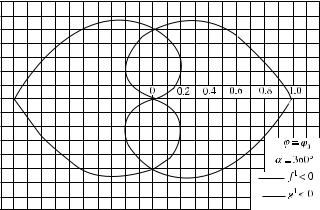
Figures 4.1 and 4.2 illustrate the behavior and beauty of functions f (1) and g(1).

4.2INTEGRAL FORM OF FUNCTIONS f (1) AND g(1)

It is well known in antenna and scattering theories that the directivity pattern of the far field can be considered as a conformal Fourier transform of the radiating/scattering sources distributed over antennas/scatterers. This is clearly seen in Equation (1.19). In this section we will establish this type of relationship between the directivity patterns f (1), g(1) and their sources js(1), jh(1) at the wedge.

The geometry of the problem is shown in Figure 3.1 and the incident wave is given by Equation (3.1). The nonuniform components of the surface sources

js(1) = u0Js(1),

jh(1) = u0Jh(1)

(4.22)

radiate the field defined by Equation (1.10). We consider first the radiation from the wedge face ϕ = 0:

eik√

(1)

= −

u0

∞

(1)

(kξ , ϕ0)dξ

∞

(x−ξ )2+y2+ζ 2

dζ ,

(4.23)

us

Js

4π

−∞

'

0

(x − ξ )2 + y2 + ζ 2

TEAM LinG

4.2 Integral form of Functions f (1) and g(1) 77

eik√

(1)

= −

u0 ∂

∞

(1)

∞

(x−ξ )2+y2+ζ 2

uh

Jh

(kξ , ϕ0)dξ

dζ .

(4.24)

4π ∂y

0

'(x − ξ )

2

+ y

2

+ ζ

2

In view of Equation (3.7),

−∞

(1)

i

∞ (1)

(1)

us

= −u0

Js

(kξ , ϕ0)H0

k((x − ξ )2

+ y2

dζ

(4.25)

4

0

and

i ∂

∞

(1)

= −u0

(1)

(1)

k((x − ξ )2 + y2

dζ .

(4.26)

uh

Jh

(kξ , ϕ0)H0

4

∂y

0

According to Equations (2.61) and (2.63), the functions Js(1) and Jh(1) decrease as (kξ )−3/2 and (kξ )−1/2, respectively, with increasing distance ξ from the edge. At a certain distance ξ = ξeffective, these functions are sufficiently small and can be approx-

imated by zero for ξ ≥ ξeff . In the far zone, where r kξeff2 , the Hankel function in Equations (4.25) and (4.26) can be replaced by its asymptotics (2.29). This leads to

the asymptotic expressions

u(1)

−

u

ei(kr+π/4) ξeff

J(1)(kξ , ϕ

)e−ikξ cos ϕ dξ

(4.27)

0 2√

0

s

2π kr

0

s

and

(1)

−u0ik sin ϕ

ei(kr+π/4)

ξeff

(1)

(kξ , ϕ0)e−ikξ cos ϕ dξ .

uh

2√

Jh

(4.28)

2π kr

0

These expressions describe the field radiated from the face ϕ = 0. By the replacement of ϕ by α − ϕ and ϕ0 by α − ϕ0, one can find the field radiated from the face ϕ = α. The total field created by both faces must be equal to that of Equations (4.12) and (4.13). By equating them we obtain the useful relationships

				1			ξeff
	f (1)(ϕ, ϕ0, α) = −							Js(1)(kξ , ϕ0)e−ikξ cos ϕ dξ
				2			0
	+				ξeff		Js(1)(kξ , α − ϕ0)e−ikξ cos(α−ϕ) dξ			(4.29)
				0
and
		ik				ξeff
g(1)	(ϕ, ϕ0, α) = −		sin ϕ				Jh(1)(kξ , ϕ0)e−ikξ cos ϕ dξ
		2		0
	+ sin(α − ϕ)					ξeff		Jh(1)(kξ , α − ϕ0)e−ikξ cos(α−ϕ) dξ	.	(4.30)
						0

TEAM LinG

= Ez(t)

78 Chapter 4 Radiation by the Nonuniform Component of Surface Sources

These expressions show that the functions f (1) and g(1) can also be interpreted as the directivity patterns of elementary diffracted waves generated (in the plane normal to the edge) by the sources distributed at the wedge along the lines normal to the edge.

4.3 OBLIQUE INCIDENCE OF A PLANE WAVE AT A WEDGE

For an oblique incidence, the relationship us(t) exists for the diffracted rays generated by the total surface currents, j(t) = j(0) + j(1). However, us(0,1) is not equal to Ez(0,1),

because of the polarization coupling in the electromagnetic PO field.

The complete equivalence uh(0,1,t) = Hz(0,1,t) exists between the acoustic and electromagnetic diffracted rays.

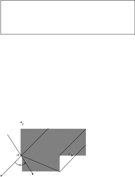
Here, we extend the results of Section 4.1 to the general case when the incident wave propagates under the oblique direction to the edge (Fig. 4.3). It is given by the equation

uinc = u0eik(x cos α˜ +y cos β+z cos γ )

(4.31)

with 0 < γ ≤ π/2. We use the “tilde-hat” for the angle α˜ to avoid possible confusion with the external angle α of the wedge.

The boundary conditions on the wedge faces are shown in Equations (2.2) and (2.3). To satisfy these conditions, the diffracted field must have the same dependence on the coordinate z as the incident wave (4.31):

ud = u(r, ϕ)eikz cos γ .

(4.32)

The substitution of this function ud into the wave equation (2.4) leads to the equation for the function u(r, ϕ),

	u(r, ϕ) + k12u(r, ϕ) = 0, with k1 = k sin γ ,		(4.33)

Figure 4.3 Oblique incidence of a plane wave at a wedge.

TEAM LinG

4.3 Oblique Incidence of a Plane Wave at a Wedge 79

where the Laplacian operator is defined by Equation (2.5). It is also expedient to represent the incident wave (4.31) in the form of Equation (3.1):

uinc = u0eikz cos γ e−ik1(x cos ϕ0+y sin ϕ0),					(4.34)
where
sin γ cos ϕ0 = − cos α˜ ,				sin γ sin ϕ0 = − cos β	(4.35)
and
tan ϕ0	=	cos β		with 0 ≤ ϕ0 < π .
			,		(4.36)
		cos α
		˜

Thus, we reduced the three-dimensional (3-D) diffraction problem for the oblique incidence to the 2-D problem for the normal incidence (γ = π/2) considered in Chapter 2. The solution for the oblique incidence can be automatically found by

simple replacements in the solution for the normal incidence. Namely, the quantity u0 should be replaced by u0eikz cos γ , the wave number k by k1 = k sin γ , and the angle

ϕ0 by ϕ0 = arctan(cos β/ cos α)˜ .

This rule has been established here for the exact solution of the wedge diffraction problem and for its asymptotics. One can show that it is also valid for the PO part of the field. First, by the substitution of the incident wave (4.34) into Equation (1.31)

we find the PO surface sources
js(0) = −u0eikz cos γ 2ik1 sin ϕ0e−ik1x cos ϕ0 ,	(4.37)
jh(0) = u0eikz cos γ 2eik1x cos ϕ0 .	(4.38)

Comparison with Equation (3.2) shows that the sources (4.37) and (4.38) satisfy the above rule for the transition from normal to oblique incidence. If the sources of the field satisfy this rule, one can expect the generated field does too. To verify that, we substitute Equations (4.37) and (4.38) into the original expressions (1.32) for the PO field:

u(0)	=		u	ik1 sin ϕ0					∞	e−ik1ξ cos ϕ0
				0
s						2π			0
(0)		= −u0				1 ∂			∞	e−ik1ξ cos ϕ0
uh
						2π		∂y	0

				eik√
∞		ikζ cos γ			(x−ξ )2+y2+(z−ζ )2
dξ	e									dζ ,
−∞			'(x − ξ )			2	+ y2	+ (z −	2
									ζ )(4.39)
				eik√
∞		ikζ cos γ			(x−ξ )2+y2+(z−ζ )2
dξ	e									dζ ,
−∞			'(x − ξ )			2	+ y2	+ (z −	2
									ζ )(4.40)

TEAM LinG

80

Chapter 4 Radiation by the Nonuniform Component of Surface Sources

or

eik√

∞

∞

u(0)

u

eikz cos γ

ik1 sin ϕ0

e−ik1ξ cos ϕ0 dξ

(x−ξ )2+y2+s2

ds,

=

eiks cos γ

s

0

2π

'

0

−∞

(x

−

ξ

)

2

+

y2

+

s2

(4.41)

eik√

(0)

1 ∂

∞

e−ik1ξ cos ϕ0 dξ

∞

(x−ξ )2+y2+s2

uh

= −u0eikz cos γ

eiks cos γ

ds.

2π ∂y

0

'(x −

2

+

y2

+

s2

−∞

ξ )

(4.42)

The integrals over the variable s still contain the wave number k for the normal

incidence and need further investigation. Let us rewrite them as

√

∞	eik			D2		s2
							ds, with D = ((x − ξ )2 + y2.
−∞ eiks cos γ						+				(4.43)
	'
			D2			s2
					+

We then return to the integral (3.8) for the Hankel function and make the following

changes: w = s, z = t, d = −ip, k = −iD, q =

p2 − t2

with D > 0 and Im q > 0.

After these manipulations it follows from (3.8) that

√

'

√

∞

2

+s

2

∞

2

+s

2

H(1)

(qD)

1

e−ist

eip

D

ds

1

eist

eip

D

ds. (4.44)

0

= iπ

2

+ s

2

π

2

+ s

2

−∞

'D

= i

−∞

'D

2

2

By setting here t = k cos γ , p = k, q = 2'p2

− t

= k sin γ = k1, we find

∞

√

iks cos γ eik

D

+s

(1)

−∞ e

ds = iπ H0

(k1D).

(4.45)

D2 + s2

This relationship allows one to rewrite the PO fields (4.41) and (4.42) in the form

'

k1 sin ϕ0

∞

k1

dξ ,

(0)

(1)

((x − ξ )2 + y2

us

= −u0eikz cos γ

e−ik1ξ cos ϕ0 H0

(4.46)

2

0

i ∂

∞

k1

dξ .

(0)

= −u0eikz cos γ

e−ik1ξ cos

(1)

((x − ξ )2 + y2

us

ϕ0 H0

(4.47)

2 ∂y

0

Comparison with expressions (3.10) and (3.11) finally confirms that the PO fields really satisfy the above rule for the transition to oblique incidence.

Thus, it has been proved that this rule is applicable both to the exact solution and to the PO approximation. Hence, this rule is also applicable to their difference, which is the field us,h(1) generated by the nonuniform component js,h(1) of the surface sources of the diffracted field. By the application of this rule to Equations (4.12) and (4.13), one can easily find the field us,h(1) generated under the oblique incidence:

(1)	u0 f	(1)		ei(k1r+π/4)				ikz cos γ
us			(ϕ, ϕ0, α)	√			e		,	(4.48)
					2π k1r

TEAM LinG

4.3 Oblique Incidence of a Plane Wave at a Wedge 81

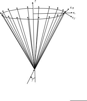
Figure 4.4 Cone of diffracted rays.

(1)	u0 g	(1)		ei(k1r+π/4)				ikz cos γ
uh			(ϕ, ϕ0, α)	√			e		,	(4.49)
					2π k1r

where the functions f (1) and g(1) are defined in Section 4.1 and the angle ϕ0 is determined by Equation (4.36).

The waves (4.48) and (4.49) have the form of conic waves and can be interpreted in terms of diffracted rays. Indeed, their eikonal

S = z cos γ + r sin γ

(4.50)

describes the phase fronts in the form of conic surfaces where S = const. The gradient of the eikonal

S = zˆ cos γ + rˆ sin γ

(4.51)

indicates the directions of the edge diffracted rays. They are distributed over a cone surface shown in Figure 4.4. The axis of this cone is directed along the edge. All rays form the same angle γ with the edge as the incident ray.

In the case of electromagnetic waves

Ezinc = E0zeikz cos γ e−ik1r cos(ϕ−ϕ0)	(4.52)
and
Hzinc = H0zeikz cos γ e−ik1r cos(ϕ−ϕ0)	(4.53)

TEAM LinG