Ufimtsev P. Fundamentals of the physical theory of diffraction (Wiley 2007)(348s) PEo

62 Chapter 3 Wedge Diffraction: The Physical Optics Field

and change the integration variable w by ξ , setting w = −k cos ξ , v = k sin ξ ,

Then,

kr cos(ξ − ϕ),

v|y| − wx =

kr cos(ξ + ϕ),

The equations

Im v > 0.

(3.17)

with ϕ < π

(3.18)

with ϕ > π .

w = −k cos ξ cosh ξ + ik sin ξ sinh ξ ,					(3.19)
v = k sin ξ cosh ξ + ik cos ξ sinh ξ
and the condition
		Im v = k cos ξ sinh ξ		> 0	(3.20)
determine the integration path F in the complex plane ξ = ξ + iξ					as shown in
Figure 3.2.
After these manipulations we obtain the following expressions:
Is =		eikr cos(ξ −ϕ)	dξ ,	with ϕ < π ,	(3.21)
	F cos ξ + cos ϕ0
Is =		eikr cos(ξ +ϕ)	dξ ,	with ϕ > π ,	(3.22)
	F cos ξ + cos ϕ0

Figure 3.2 Integration contour F in the complex plane ξ = ξ + iξ .

TEAM LinG

	3.2 Conversion of the PO Integrals to the Canonical Form 63
and
Ih = F		eikr cos(ξ −ϕ) sin ξ	dξ ,	with ϕ < π ,	(3.23)
		cos ξ + cos ϕ0
Ih = F		eikr cos(ξ +ϕ) sin ξ	dξ ,	with ϕ > π ,	(3.24)
		cos ξ + cos ϕ0

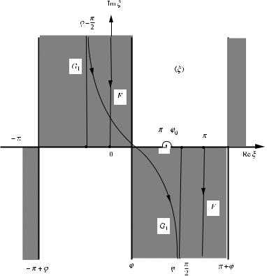
where, as is shown in Figure 3.2, the integration contour F skirts above the pole

ξ = π − ϕ0.

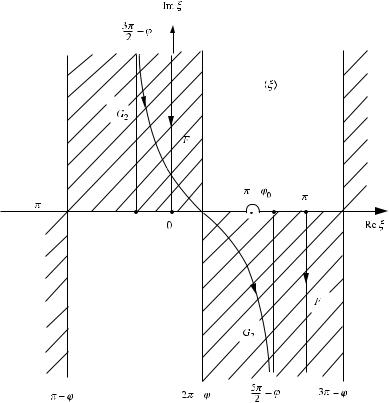
In Figures 3.3 and 3.4, we introduce two additional contours G1 and G2, related to the cases ϕ < π and ϕ > π , respectively. In the dashed regions of these figures, the relations Im cos(ξ − ϕ) > 0 and Im cos(ξ + ϕ) > 0 are valid, which guarantees the convergence of integrals Is and Ih. We then apply the Cauchy residue theorem

Figure 3.3 Integration contours F and G1 for the case ϕ < π . In the shaded regions, Im cos(ξ − ϕ) > 0.

TEAM LinG

64 Chapter 3 Wedge Diffraction: The Physical Optics Field

Figure 3.4 Integration contours F and G2 for the case ϕ > π . In the shaded regions, Im cos(ξ + ϕ) > 0.

to the integrals over the closed contours F − G1,2 (they are closed at the infinity, ξ = ±∞) and obtain

Is =	eikr cos(ξ −ϕ)				dξ +	2π i		e−ikr cos(ϕ+ϕ0),	with 0 ≤ ϕ ≤ π − ϕ0,
	cos ξ	+	cos ϕ	0		sin ϕ	0
G1

(3.25)

Is =

Is =

and

Is =

G1

G2

G2

eikr cos(ξ −ϕ)					dξ ,	with π − ϕ0 < ϕ < π ,		(3.26)
cos ξ + cos ϕ0
eikr cos(ξ +ϕ)					dξ ,	with π < ϕ < π + ϕ0,		(3.27)
cos ξ + cos ϕ0
eikr cos(ξ +ϕ)					dξ +	2π i	e−ikr cos(ϕ−ϕ0),	with π + ϕ0 ≤ ϕ ≤ 2π .
cos ξ	+	cos ϕ	0			sin ϕ
						0		(3.28)

TEAM LinG

3.2 Conversion of the PO Integrals to the Canonical Form 65

In these equations, we change with integration variable ξ by ζ + ϕ in the region 0 ≤ ϕ < π , and by ζ + 2π − ϕ in the region π < ϕ < 2π . As a result, the integrals in Equations (3.25) to (3.28) are transformed into the integrals over the contour D0 shown in Figure 2.6:

	eikr cos(ξ −ϕ)	dξ =		eikr cos ζ dζ		with 0 ≤ ϕ < π
					,		(3.29)
G1	cos ξ + cos ϕ0		D0	cos ϕ0 + cos(ζ + ϕ)
and
	eikr cos(ξ +ϕ)	dξ =		eikr cos ζ dζ		with π ≤ ϕ < 2π .
					,		(3.30)
G2	cos ξ + cos ϕ0		D0	cos ϕ0 + cos(ζ − ϕ)

We omit similar transformations for integral Ih and present only their results:

Ih =

Ih =

Ih =

Ih =

eikr cos ζ sin(ζ + ϕ)

dζ

+

2π ie−ikr cos(ϕ+ϕ0),

with 0

≤

ϕ

≤

π

−

ϕ

,

cos ϕ0 + cos(ζ + ϕ)

D0

0

(3.31)

eikr cos ζ sin(ζ + ϕ)

dζ ,

with π

−

ϕ

0

≤

ϕ < π ,

(3.32)

D0

cos ϕ0 + cos(ζ + ϕ)

eikr cos ζ sin(ζ − ϕ)

dζ ,

with π

≤

ϕ

≤

π

+

ϕ

,

(3.33)

cos ϕ0 + cos(ζ − ϕ)

D0

0

eikr cos ζ sin(ζ − ϕ)

dζ

+

2π ie−ikr cos(ϕ−ϕ0),

with π

+

ϕ

0 ≤

ϕ

≤

2π .

D0

cos ϕ0 + cos(ζ − ϕ)

(3.34)

Finally one can represent the scattered field in the following form:

(0)		−u0e−ikr cos(ϕ+ϕ0),		with	0 ≤ ϕ ≤ π − ϕ0
us	= u0vs+(kr, ϕ, ϕ0) + 0,			with π		−	ϕ0 < ϕ < π ,
	= u0vs−(kr, ϕ, ϕ0) +
(0)		0,	u0e−ikr cos(ϕ−ϕ0),	with π		≤	ϕ ≤ π + ϕ0
us		−		with π			ϕ0 < ϕ < 2π ,
and						+
(0)		u0e−ikr cos(ϕ+ϕ0),		with 0	≤	ϕ ≤ π − ϕ0
uh	= u0vh+(kr, ϕ, ϕ0) + 0,			with π		ϕ0 < ϕ < π ,
	= u0vh−(kr, ϕ, ϕ0) +				−
(0)		0,	u0e−ikr cos(ϕ−ϕ0),	with π		≤	ϕ ≤ π + ϕ0
uh		−		with π			ϕ0 < ϕ < 2π ,
						+

(3.35)

(3.36)

(3.37)

(3.38)

TEAM LinG

66 Chapter 3 Wedge Diffraction: The Physical Optics Field

where

v±(kr, ϕ, ϕ )

=

i sin ϕ0

eikr cos ζ

dζ ,

(3.39)

s

0

2π

D0

cos ϕ0 + cos(ζ ± ϕ)

and

v±(kr, ϕ, ϕ

)

1

eikr cos ζ sin(ζ ± ϕ)

dζ .

(3.40)

0

= ± i2π

h

D0

cos ϕ0 + cos(ζ ± ϕ)

The above expressions for us(0) and uh(0) determine the PO field scattered by the face ϕ = 0 of the wedge. They are valid under the condition 0 ≤ ϕ0 < α − π .

However, in the case α − π < ϕ0 < π , the other face (ϕ = α) is also illuminated and generates the additional scattered field. This field is also determined by Equations (3.35) to (3.38), where one should replace ϕ by α − ϕ and ϕ0 by α − ϕ0. Thus, the PO field us(0) scattered in this case by both faces of the wedge is described by the following equations:

u(0)

=

u

0[

v+(kr, ϕ, ϕ )

+

v−(kr, α

−

ϕ, α

−

ϕ

)

]

s

s

0

s

0

−u0e−ikr cos(ϕ+ϕ0),

with 0 ≤ ϕ ≤ π − ϕ0

π .

(3.41)

+ 0,

with π

−

ϕ0

< ϕ < α

−

u(0)

=

u

0[

v+(kr, ϕ, ϕ )

+

v+(kr, α

−

ϕ, α

−

ϕ

)

]

,

with α

−

π < ϕ < π ,

s

s

0

s

0

(3.42)

u(0)

=

u

0[

v−(kr, ϕ, ϕ )

+

v+(kr, α

−

ϕ, α

−

ϕ

)

]

,

with π < ϕ < 2α

−

π

−

ϕ

,

s

s

0

s

0

0

(3.43)

and

u(0)

=

u

0[

v−(kr, ϕ, ϕ )

+

v+(kr, α

−

ϕ, α

−

ϕ

)

]

s

s

0

s

0

− u0e−ikr cos(2α−ϕ−ϕ0),

with 2α − π − ϕ0 < ϕ < α.

(3.44)

Similar equations are valid for the field uh(0) in the case α − π < ϕ0 < π :

uh(0) = u0[vh+(kr, ϕ, ϕ0) + vh−(kr, α − ϕ, α − ϕ0)]

u0e−ikr cos(ϕ+ϕ0),

with 0

ϕ ≤ π − ϕ0

π ,

(3.45)

+ 0,

with π ≤

ϕ0 < ϕ < α

−

−

TEAM LinG

cos ϕ + cos ϕ0

√

	3.3 Ray Asymptotics for the PO Diffracted Field 67
uh(0) = u0[vh+(kr, ϕ, ϕ0) + vh+(kr, α − ϕ, α − ϕ0)],		with α − π < ϕ < π ,	(3.46)
uh(0) = u0[vh−(kr, ϕ, ϕ0) + vh+(kr, α − ϕ, α − ϕ0)],		with π < ϕ < 2α − π − ϕ0,
			(3.47)
uh(0) = u0[vh−(kr, ϕ, ϕ0) + vh+(kr, α − ϕ, α − ϕ0)]
+ u0e−ikr cos(2α−ϕ−ϕ0),	with 2α − π − ϕ0 < ϕ < α.		(3.48)

As is seen in Equations (3.41) to (3.48), the PO scattered field consists of the reflected plane waves and the diffracted part described by functions vs± and vh±. Simple asymptotic expressions for the functions vs,h± and for the diffracted field are derived in the next section.

3.3 RAY ASYMPTOTICS FOR THE PO DIFFRACTED FIELD

The relationships us = Ez and uh = Hz exist between the acoustic and electromagnetic

fields studied in this section.

Again, as in √Section 2.4, we introduce in the integrals (3.39) and (3.40) the new variable s = 2eiπ/4 sin ζ2 and transform functions vs,h± as

v±(kr, ϕ, ϕ )		=	sin ϕ0						ei(kr+π/4)
			√
s	0				2	π
v±(kr, ϕ, ϕ )			1							ei(kr+π/4)
		= √
h	0						2	π

∞e−krs2 ds

−∞ [cos ϕ0 + cos(ζ ± ϕ)] cos ζ , 2

∞sin(ζ ± ϕ)e−krs2 ds

−∞ [cos ϕ0 + cos(ζ ± ϕ)] cos ζ . 2

Then the standard saddle point technique leads to the asymptotic expressions

v±(kr, ϕ, ϕ )

sin ϕ0

ei(kr+π/4)

,

cos ϕ + cos ϕ0

√

s

0

2π kr

and

v±(kr, ϕ, ϕ )

−

sin ϕ

ei(kr+π/4)

.

√

h

0

2π kr

(3.49)

(3.50)

(3.51)

(3.52)

These asymptotics are valid under the conditions kr| cos(ϕ ± ϕ0)/2| 1, that is, away from the geometrical optics boundaries, where the diffracted field has a ray structure and can be interpreted in terms of edge diffracted rays.

TEAM LinG

68 Chapter 3 Wedge Diffraction: The Physical Optics Field

In view of Equations (3.51) and (3.52), the ray asymptotics for the diffracted part of the fields (3.41) to (3.44) and (3.45) to (3.48) can be written in the following form:

(0)d	u0 f	(0)			ei(kr+π/4)
us				(ϕ, ϕ0)	√						(3.53)
						2π kr
and
(0)d	u0 g		(0)		ei(kr+π/4)
uh				(ϕ, ϕ0)	√					.	(3.54)
							2π kr

The directivity patterns of these diffracted rays are different for the situations with one or two illuminated faces. In the case 0 < ϕ0 < α − π , when only the face ϕ = 0 is illuminated by the incident wave,

f (0)(ϕ, ϕ0) =

sin ϕ0

g(0)(ϕ, ϕ0) = −

sin ϕ

,

.

cos ϕ + cos ϕ0

cos ϕ + cos ϕ0

However, if both faces are illuminated (α − π < ϕ0 < π ),

f (0)(ϕ, ϕ

)

sin ϕ0

sin(α − ϕ0)

= cos ϕ + cos ϕ0

+ cos(α − ϕ) + cos(α − ϕ0)

0

and

g(0)(ϕ, ϕ

)

sin ϕ

sin(α − ϕ)

.

= − cos ϕ + cos ϕ0

− cos(α − ϕ) + cos(α − ϕ0)

0

(3.55)

(3.56)

(3.57)

It is seen that these functions are singular at the boundaries of reflected plane waves, where ϕ = π ± ϕ0 or ϕ = 2α − π − ϕ0. The asymptotics of the PO diffracted field, which are uniformly valid around the wedge, can be easily derived by the application of the Pauli technique demonstrated in Sections 2.5 and 2.6. We do not consider them here, because our main purpose in the canonical wedge diffraction problem is the calculation of the field generated by the nonuniform component of the surface sources.

PROBLEMS

3.1 Analyze the accuracy of the PO approximation. Compute and plot the relative error

δf (0)(ϕ, ϕ0, α) = |F(ϕ, ϕ0, α) − 1| · 100%,

where

F(ϕ, ϕ0, α) = f (0)(ϕ, ϕ0)/f (ϕ, ϕ0, α).

TEAM LinG

Problems 69

Consider these two examples:

(a) α = 270◦, ϕ0 = 45◦, 0 ≤ ϕ ≤ α, (b) α = 360◦, ϕ0 = 45◦, 0 ≤ ϕ ≤ α.

Prove analytically that F(π ± ϕ0, ϕ0, α) = 1. Formulate your conclusion regarding δf (0).

3.2 Analyze the accuracy of the PO approximation. Compute and plot the relative error

δg(0)(ϕ, ϕ0, α) = |G(ϕ, ϕ0, α) − 1| · 100%,

where

G(ϕ, ϕ0, α) = g(0)(ϕ, ϕ0)/g(ϕ, ϕ0, α). Consider these two examples:

(a) α = 270◦, ϕ0 = 45◦, 0 ≤ ϕ ≤ α, (b) α = 360◦, ϕ0 = 45◦, 0 ≤ ϕ ≤ α.

Prove analytically that G(π ± ϕ0, ϕ0, α) = 1. Formulate your conclusion regarding δg(0).

3.3The Sommerfeld function f (ϕ, ϕ0, α) satisfies the reciprocity principle, but its PO approximation f (0)(ϕ, ϕ0) does not. Analyze the PO deviations from the reciprocity principle. Compute the relative level of these deviations,

df (ϕ, ϕ0) = |F(ϕ, ϕ0, α) − F(ϕ0, ϕ, α)| · 100%,

where

F(ϕ, ϕ0, α) = f (0)(ϕ, ϕ0)/f (ϕ, ϕ0, α).

Investigate the case with α = 350◦, set ϕ = ϕ0 = 70◦. Prepare a (6 × 6) square table with numerical data for the deviations df . Formulate your conclusion.

3.4The Sommerfeld function g(ϕ, ϕ0, α) satisfies the reciprocity principle, but its PO approximation g(0)(ϕ, ϕ0) does not. Analyze the PO deviations from the reciprocity principle. Compute the relative level of these deviations,

dg(ϕ, ϕ0) = |G(ϕ, ϕ0, α) − G(ϕ0, ϕ, α)| · 100%,

where

G(ϕ, ϕ0, α) = g(0)(ϕ, ϕ0, α)/g(ϕ, ϕ0, α).

Investigate the case with α = 350◦, set ϕ = ϕ0 = 70◦. Prepare a (6 × 6) square table with numerical data for the deviations dg. Formulate your conclusion.

TEAM LinG

TEAM LinG

= Ez(1)

= Hz(1)

Chapter 4

Wedge Diffraction:

Radiation by the Nonuniform

Component of Surface Sources

The relationships us(1) and uh(1) exist between the acoustic and electromagnetic fields generated by the nonuniform sources j(1). An exception exists for an oblique incidence (see Section 4.3).

We have now reached the moment when we can construct the integral and asymptotic representations for the field radiated by the nonuniform component of the surface sources, which are induced at the wedge by the incident wave. The exact expressions for the total field generated around the wedge have been derived in Chapter 2. The Physical Optics (PO) part of this field (which is generated by the uniform component of the surface sources) has been studied in Chapter 3. The contribution to the diffracted field by the nonuniform component is the difference between the exact total field and its PO part. This contribution is investigated in this chapter.

4.1INTEGRALS AND ASYMPTOTICS

According to the exact solution (see Equations (2.40), (2.41), and (2.52) to (2.57)), the total field around the wedge consists of the diffracted and geometrical optics parts

us,ht = us,hd + us,hgo ,

(4.1)

where us,hd is described by the functions v(kr, ψ ), and us,hgo is the sum of the incident and reflected plane waves. Equations (3.35) and (3.36), (3.37) and (3.38), (3.41) to

(3.44), and (3.45) to (3.48) represent the scattered field in the PO approximation.

Fundamentals of the Physical Theory of Diffraction. By Pyotr Ya. Ufimtsev

Copyright © 2007 John Wiley & Sons, Inc.

71

TEAM LinG