Ufimtsev P. Fundamentals of the physical theory of diffraction (Wiley 2007)(348s) PEo

32 Chapter 1 Basic Notions in Acoustic and Electromagnetic Diffraction Problems

(c) Apply the optical theorem (5.16) to the field in the direction φ = π − φ0 and provide the geometrical interpretation of the total reflecting cross-section.

(d) Compute and plot the directivity pattern of the reflected field, setting a = 2λ, φ0 = 45◦. What are the interesting properties of this field?

1.6Solve the problem similar to Problem 1.5, but for a hard strip.

1.7Suppose that the incident wave uinc = u0 exp[ik(x cos φ0 + y sin φ0)] hits a soft strip as shown in Figure 5.1. Use Equation (1.72) and calculate the shadow radiation part of the PO field scattered by this strip.

(a) Express the integral over the variable ζ through the Hankel function (3.7), apply its asymptotic approximation (2.29), and calculate the far field (r ka2) in closed form.

(b) Estimate the field in the directions φ = φ0, φ = π − φ0, and φ = π + φ0.

(c) Apply the optical theorem (5.16) to the field in the direction φ = φ0 and give the geometrical interpretation of the total power of the shadow radiation.

(d) Compute and plot the directivity pattern of the shadow radiation, setting a = 2λ, φ0 = 45◦. What are the interesting properties of this field?

1.8Is the difference between the reflected parts of the PO field scattered by soft and hard objects (of the same shape and size) illuminated by the same incident wave.

1.9Is any difference between the shadow parts of the PO field scattered by soft and hard objects (of the same shape and size) illuminated by the same incident wave.

1.10The incident wave Ezinc = E0z exp[ik(x cos φ0 + y sin φ0)] hits a perfectly conducting strip as shown in Figure 5.1. Calculate the reflected part of the PO scattered field.

(a) Start with Equations (1.87), (1.88) and (1.89). Apply je,refl		n	Hinc, jm,refl	=
ˆ ×	inc	= ˆ ×
	E . Prepare the integral expression for the reflected field.
n

(b) Express the integral over the variable ζ through the Hankel function (3.7), apply its asymptotic approximation (2.29), and express the far field (r ka2) in closed form.

(c) Estimate the field in the directions φ = φ0, φ = π − φ0, φ = π + φ0, and φ = −φ0. (d) Apply the optical theorem (5.16) to the field in the direction φ = π − φ0 and provide

the geometrical interpretation of the total reflecting cross-section.

(e) Compute and plot the directivity pattern of the reflected field, setting a = 2λ, φ0 = 45◦. What are the interesting properties of this field?

1.11The incident wave Ezinc = E0z exp[ik(x cos φ0 + y sin φ0)] hits a perfectly conducting strip as shown in Figure 5.1. Calculate the shadow radiation part of the PO scattered field.

(a) Start with Equations (1.87), (1.88) and (1.89). Apply

	je,sh	n	Hinc, jm,sh	n	Einc.
		= ˆ ×		= − ˆ ×
	Prepare the integral expression for the shadow radiation.
(b)	Express the integral over the variable ζ through the Hankel function (3.7), apply its
	asymptotic approximation (2.29), and calculate the far field (r					ka2) in closed form.
(c)	Estimate the field in the directions φ = φ0, φ = π − φ0, and φ = π + φ0.

(d)	Apply the optical theorem (5.16) to the field in the direction φ = φ0 and provide the
	geometrical interpretation of the total power of the shadow radiation.
(e)	Compute and plot the directivity pattern of the reflected field, setting a = 2λ,
	φ0 = 45◦. What are the interesting properties of this field?

TEAM LinG

Chapter 2

Wedge Diffraction: Exact

Solution and Asymptotics

The relationships us = Ez and uh = Hz exist between the acoustic and electromagnetic fields in the 2-D wedge diffraction problem. Here, Ez and Hz are the components

(of vectors E and H) that are parallel to the edge of the wedge.

2.1CLASSICAL SOLUTIONS

Diffraction at a wedge with a straight edge and infinite planar faces is an appropriate canonical problem to derive asymptotic expressions for the edge waves scattered from arbitrary curved edges. In the particular case of the wedge, which is a semi-infinite half-plane, the exact solution of this canonical problem was found by Sommerfeld (1896), who constructed so-called branched wave functions. Analysis of this work performed in Ufimtsev (1998) shows that Sommerfeld also developed almost everything that was necessary to obtain the solution for the wedge with an arbitrary angle between its faces. However, he missed the last step that led directly to the solution. This more general solution was found by Macdonald (1902) with the classical method of separation of variables in the wave equation. Later on, Sommerfeld also constructed the solution of the wedge diffraction problem by his method of branched wave functions and derived simple asymptotic expressions for the edge-diffracted waves (Sommerfeld, 1935).

Because the wedge diffraction problem is the basis for the construction of PTD, its solution is considered here in detail. First we derive this solution in the form of infinite series and then convert it to the Sommerfeld integrals convenient for asymptotic analysis. The material of this chapter, with the exception of Sections 2.6 and 2.7, is a scalar version of the theory developed by the author for electromagnetic waves (Ufimtsev, 1962).

Fundamentals of the Physical Theory of Diffraction. By Pyotr Ya. Ufimtsev

Copyright © 2007 John Wiley & Sons, Inc.

33

TEAM LinG

34 Chapter 2 Wedge Diffraction: Exact Solution and Asymptotics

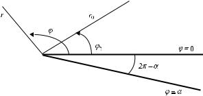
Figure 2.1 A wedge is excited by a filamentary source located at the line r = r0, ϕ = ϕ0.

The geometry of the problem is shown in Figure 2.1. A wedge with infinite planar faces ϕ = 0 and ϕ = α is located in a homogeneous medium. It is excited by a cylindrical wave. The source of this wave is a radiating filament with coordinates

r= r0, ϕ = ϕ0. This is a two-dimensional problem where ∂/∂z ≡ 0. The field outside the wedge (0 ≤ ϕ ≤ α) satisfies the wave equation

u + k2u = I0δ(r − r0, ϕ − ϕ0)	(2.1)
and the boundary conditions
us = 0	(2.2)
or
∂uh/∂n = 0	(2.3)

on the faces ϕ = 0 and ϕ = α. In the case of electromagnetic waves, these boundary conditions are appropriate for the perfectly conducting wedge, and function us

represents the z-component of electric field intensity E, while function uh is the

z-component of magnetic field intensity H. In the case of acoustic waves, condition (2.2) relates to the acoustically soft wedge, and (2.3) to the acoustically hard wedge.

Outside the immediate vicinity of the source, the field u satisfies the homogeneous wave equation

u + k2u = 0.

(2.4)

For the two-dimensional problem, the Laplacian operator is defined by

=

∂2

+

1 ∂

+

1 ∂2

.

(2.5)

∂r2

r

∂r

r2

∂ϕ2

Using the classical method of separation of variables, we set in Equation (2.4)

u = R(r) (ϕ)

(2.6)

TEAM LinG

2.1 Classical Solutions

35

and substitute this u into Equation (2.4). After simple manipulations, the latter can be separated into two equations:

	d2R 1 dR							v2
		+				+	1 −		l	R = 0, with x = kr,	(2.7)
	dx2		x		dx				x2
and
							d2		+ vl2 = 0.		(2.8)
							dϕ2

The function and the separation constants vl are determined from the boundary conditions.

In the case of soft boundary conditions, according to Equations (2.2) and (2.8),

= {sin vl ϕ}, vl = l	π
	α , l = 1, 2, 3, . . . ,	(2.9)

and, in the case of hard boundary conditions, in accordance with Equations (2.3) and (2.8),

= {cos vl ϕ},	vl = l	π			l = 0, 1, 2, 3, . . . .
				,		(2.10)
		α
The Bessel and Hankel functions
	Jvl (kr)
	R = Hv(1l		)(kr)			(2.11)

represent the solution of the radial equation (2.7). The Bessel functions Jvl (kr) can be used in the region r ≤ r0, because they are finite at the edge r = 0, and the Hankel functions are appropriate in the region r ≥ r0, because they satisfy Sommerfeld’s radiation condition at infinity:

du

lim √r

− iku = 0, with r → ∞.

(2.12)

dr

Hence, the solutions of Equation (2.4) can be written as

s

∞

(kr)Hv(1l

)(kr0) sin vl ϕ0 sin vl ϕ,

with r ≤ r0

l

1 al Jvl

=

∞

u

=

(2.13)

(1)

(kr) sin vl ϕ0 sin vl ϕ,

with r ≥ r0

1 al Jvl

(kr0)Hvl

l

=

h

∞

(kr)Hv(1l

)(kr0) cos vl ϕ0 cos vl ϕ,

with r ≤ r0

l

0 bl Jvl

=

∞

u

=

(2.14)

(1)

(kr) cos vl ϕ0 cos vl ϕ,

with r ≥ r0

0 bl Jvl

(kr0)Hvl

l

=

TEAM LinG

36 Chapter 2 Wedge Diffraction: Exact Solution and Asymptotics

Figure 2.2 The integration contour L in the Green theorem (2.15).

These expressions satisfy the boundary conditions, as well as the reciprocity principles; that is, they do not change after interchanging r and r0, ϕ and ϕ0.

The unknown coefficients al and bl can be found by applying the Green theorem

∂u
L ∂n dl = S u ds, ds = r dr dϕ	(2.15)

to the fields us and uh in the region S bounded by the contour L shown in Figure 2.2. This contour consists of two arcs r = r0 − ε, r = r0 + ε and two radial sides

ϕ = ϕ0 − ψ , ϕ = ϕ0 + ψ .

Substitute us,h into (2.15), take into account that, according to Equation (2.1),

u = −k2u + I0δ(r − r0, ϕ − ϕ0),

(2.16)

and let ε tend to zero. It is clear that

S us,h ds −→ 0

when S −→ 0,

(2.17)

as the Bessel and Hankel functions are finite at r = r0 > 0.

As a result, the Green formula for us,h transforms into

ϕ0

+ψ

∂r

r r0 0 −

∂r

r r0

0 r0 dϕ

ϕ0

ψ

∂us,h

∂us,h

−

+

= +

+

= −

= I0

ϕ0 ψ

r0 ε

with ε → 0.

ϕ0−ψ

dϕ lim

δ(r − r0, ϕ − ϕ0)r dr,

(2.18)

r0−ε

The two-dimensional Delta-function in polar coordinates equals

1

− ϕ0),

δ(r − r0, ϕ − ϕ0) = δ(r − r0)

δ(ϕ

(2.19)

r

TEAM LinG

2.1 Classical Solutions 37

therefore

ϕ0

ψ

∂us,h

∂us,h

r0 dϕ = I0

ϕ0

ψ

+ψ

−

+ψ δ(ϕ − ϕ0)dϕ. (2.20)

ϕ0

∂r

r

r0 0

∂r

r

r0 0

ϕ0

−

= +

= −

−

Equation (2.20) is valid for arbitrary limits of integration. This is possible if the integrands in the left and right sides are equal to each other:

∂us,h		= +		∂us,h		= −	1
∂r	r	r0 0	−	∂r	r	r0 0	=	r0	I0δ(ϕ − ϕ0).	(2.21)

This equation can be used to determine the unknown coefficients al and bl in the expressions (2.13) and (2.14).

To do this, we substitute us of Equation (2.13) into Equation (2.21), multiply both sides by sin vt ϕ, where vt = tπ/α, and integrate them over ϕ from 0 to α. Note that

			1
0	=
α sin vl ϕ sin vt ϕ dϕ		0,			α,
			2

and obtain

with l = t

with l =t t = 1, 2, 3, . . . ,

α				d				d
kr0		al	Jvl (kr0)		Hv(1l	)(kr0) − Hv(1l	)(kr0)		Jvl (kr0) = I0.
	2			dkr0				dkr0

The expression inside the brackets is the Wronskian

	d					d		2i
W [Jv (x), Hv(1)(x)] = Jv (x)		Hv(1)(x) − Hv(1)(x)					Jv (x) =		.
	d x					d x		π x
From Equations (2.23) and (2.24) it follows that
			=	π
		al			I0.
				iα

(2.22)

(2.23)

(2.24)

(2.25)

In the case of the hard boundary conditions, we carry out similar manipulations. Substitute uh of Equation (2.14) into Equation (2.21), multiply both sides by cos vt ϕ, and integrate over ϕ from 0 to α. As a result, we obtain

bl = εl	π		with ε0 =	1		= ε2	= ε3 = · · · = 1.
		I0,			, ε1			(2.26)
	iα			2

Thus, the coefficients al and bl are found, and the functions us,h are completely determined. Now we can write the final expressions for the total field excited by the external filamentary source.

TEAM LinG

38 Chapter 2

Wedge Diffraction: Exact Solution and Asymptotics

In the case of soft boundary conditions, the field us is described by the following

expressions

π

∞

I0

Jvl (kr)Hv(1l )(kr0) sin vl ϕ0 sin vl ϕ,

with r ≤ r0

s

=

∞

π

l

u

=

1

. (2.27)

=

(1)

(kr) sin vl ϕ0 sin vl ϕ,

with r ≥ r0

1 Jvl (kr0)Hvl

iα I0 l

In the case of hard boundary conditions, the field uh is determined by

π

∞

I0

εl Jvl (kr)Hv(1l )(kr0) cos vl ϕ0 cos vl ϕ,

with r ≤ r0

h

=

∞

π

l

u

=

0

(2.28)

=

(1)

with r ≥ r0.

0

εl Jvl (kr0)Hvl

(kr) cos vl ϕ0 cos vl ϕ,

iα I0 l

These expressions relate to the excitation of the field by a cylindrical wave, with a source term I0δ(r − r0, ϕ − ϕ0) around the wedge in the region 0 ≤ ϕ ≤ α, 0 ≤ r ≤ ∞. They can be modified for excitation by a plane wave.

2.2 TRANSITION TO THE PLANE WAVE EXCITATION

For the Hankel functions with large arguments (kr0 → ∞), one can use the asymptotic expression

	)(kr0)	2			π	π	π
Hv(1l			ei(kr0	−	2 vl −	4 ) ≈ H0(1)(kr0)e−i	2 vl .	(2.29)
		π kr0

The field Equations (2.27) and (2.28) can then be rewritten for the region r < r0 as

	π		∞	π
us =		I0H0(1)(kr0)		e−i 2 vl Jvl (kr) sin vl ϕ0 sin vl ϕ,	(2.30)
	iα		l=1
	π		∞	π
uh =		I0H0(1)(kr0)		εl e−i 2 vl Jvl (kr) cos vl ϕ0 cos vl ϕ,	(2.31)
	iα		l=0

TEAM LinG

or

us =

uh =

			2.2 Transition to the Plane Wave Excitation 39
π		∞	π
	I0H0(1)(kr0)		e−i 2 vl Jvl (kr)[cos vl (ϕ − ϕ0) − cos vl (ϕ + ϕ0)], (2.32)
2iα		l=0
π		∞	π
	I0H0(1)(kr0)		εl e−i 2 vl Jvl (kr)[cos vl (ϕ − ϕ0) + cos vl (ϕ + ϕ0)].
2iα		l=0

(2.33)

To clarify these expressions, we consider the solution of the wave equation (2.1) in the free infinite homogeneous medium, without the scattering wedge. For this problem, it is convenient to use the new polar coordinates (ρ, φ) with the origin at the radiating source (r0, ϕ0). It is clear that due to the azimuthal symmetry of the problem, its solution is a function of only one variable, u = u(ρ). In addition, as the wave equation is the differential equation of second order, its solution, in general, is the sum of two fundamental solutions of the related homogeneous equation:

u(ρ) = c1H0(1)(kρ) + c2H0(2)(kρ),	(2.34)
with constants c1 and c2. We retain here only the first term,
u(ρ) = c1H0(1)(kρ),	(2.35)

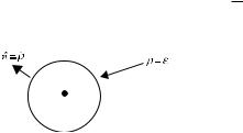
because the second term, with H0(2)(kρ), does not satisfy the Sommerfeld radiation condition (2.12) and represents a nonphysical wave incoming from infinity. The constant c1 is found again with the Green theorem (2.15) applied to the circular region S of a small radius ε and with the center at ρ = 0 (Fig. 2.3).

For small values kρ 1, the function u(kρ) and its normal derivative du/dn = du/dρ (at the boundary of the region S) are described by the asymptotic approximations

i2			du(ρ)		i2
u(ρ) ≈ c1		ln(kρ),		≈ c1		,	with kρ 1.	(2.36)
	π		dρ		πρ

By substitution of these quantities into the Green theorem and taking the limit with ε → 0, we find c1 = I0/i4 and

1
u(ρ) = i4 I0H0(1)(kρ).	(2.37)

Figure 2.3 A circular region (0 ≤ ρ ≤ ε, 0 ≤ φ ≤ 2π ) with the radiating source at the center.

TEAM LinG

40 Chapter 2 Wedge Diffraction: Exact Solution and Asymptotics

This solution explains the physical meaning of the factor in front of the series in Equations (2.32) and (2.33). It actually represents the field of the incident wave on the edge of the wedge

u0 =	1
	4i I0H0(1)(kr0).	(2.38)

When r0 → ∞ and I0 → ∞, this field can be interpreted as the plane wave traveling to the wedge from the direction ϕ = ϕ0:

uinc = u0e−ikr cos(ϕ−ϕ0).

(2.39)

As a result, one can rewrite Equations (2.32) and (2.33) in the classical Sommerfeld form (Sommerfeld, 1935):

us = u0 · [u(kr, ϕ − ϕ0) − u(kr, ϕ + ϕ0)]			for uinc = u0e−ikr cos(ϕ−ϕ0)	(2.40)
uh = u0 · [u(kr, ϕ − ϕ0) + u(kr, ϕ + ϕ0)]				(2.41)
where		∞
	2π
u(kr, ψ ) =	α	εl e−i(π/2)vl Jvl (kr) cos vl ψ .		(2.42)
		l=0

Equations (2.40) to (2.42) finally determine the total field generated by the incident plane wave in the presence of the perfectly reflecting wedge.

2.3 CONVERSION OF THE SERIES SOLUTION TO THE SOMMERFELD INTEGRALS

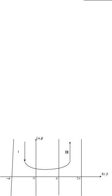
In his work Sommerfeld (1935) presented the solution of the wedge diffraction problem in integral form and then transformed it into infinite series. Here, we will perform a reverse procedure, and convert the infinite series (2.40) and (2.41) into integrals. To do this, we use the following expression of the Bessel function (Sommerfeld, 1935):

			1		III
	J(kr)	=			ei[kr cos β+vl (β−π/2)] dβ,	(2.43)
	vl		2π		I

where the integration contour is shown in Figure 2.4. Then the function u(kr, ψ ) can be represented as

	1	III	∞	∞
u(kr, ψ ) =	2α	I	eikr cos β 1 +	eivl (β−π +ψ ) + eivl (β−π −ψ )	dβ, (2.44)
			l=1	l=1

TEAM LinG

2.3 Conversion of the Series Solution to the Sommerfeld Integrals 41

with vl = lπ/α. Here, the series are geometrical leads to

	1	III	eikr cos β	1
u(kr, ψ ) =					−
	2α	I		1 − ei πα (β−π +ψ )

progressions. Their summation

1	dβ. (2.45)
1 − e−i πα (β−π −ψ )

With a new variable β			= β − π , this becomes
u(kr, ψ ) =	1	III	e−	ikr cos β		1	−	1	dβ . (2.46)
	2α	I				1 − ei πα (β +ψ )		1 − e−i πα (β −ψ )

Here, the integration contour is shifted by −π compared to the contour shown in Figure 2.4. According to the difference inside the brackets, the function u(kr, ψ ) can be represented as the sum of two integrals. In the integral related to the first term inside the brackets, we replace β by β. In the integral related to the second term inside the brackets, we change β by −β. As a result, we arrive at the Sommerfeld integral (Sommerfeld, 1935)

u(kr, ψ ) =	1			e−ikr cos β				dβ.	(2.47)
	2α	C 1		− e	i πα (β	+	ψ )

The integration contour C, consisting of two branches, is shown in Figure 2.5. The integrand of u(kr, ψ ) possesses the first-order poles

βm = 2αm − ψ , with m = 0, ±1, ±2, ±3, . . . .

(2.48)

Application of the Cauchy theorem to the integral over the closed contour C–D (Fig. 2.5) results in

u(kr, ψ ) = v(kr, ψ ) + e−ikr cos ψ ,	with −π < ψ < π ,
u(kr, ψ ) = v(kr, ψ ), with π < ψ < 2α − π ,		(2.49)
u(kr, ψ ) = v(kr, ψ ) + e−ikr cos(2α−ψ ),	with 2α − π < ψ < 2α + π ,

Figure 2.4 Integration contour in Equation (2.43).

TEAM LinG