Ufimtsev P. Fundamentals of the physical theory of diffraction (Wiley 2007)(348s) PEo

u(kr, ϕ − ϕ0) = v(kr, ϕ − ϕ0) + e−ikr cos(ϕ−ϕ0) u(kr, ϕ + ϕ0) = v(kr, ϕ + ϕ0) + e−ikr cos(ϕ+ϕ0)

42 Chapter 2 Wedge Diffraction: Exact Solution and Asymptotics

Figure 2.5 Integration contours in Equations (2.47) and (2.50).

where

v(kr, ψ ) =	1			e−ikr cos β				dβ.	(2.50)
	2α	D 1		− e	i πα (β	+	ψ )

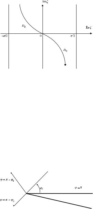
The integration contour D consists of two branches (Fig. 2.5). In the integral over the left branch, we replace the variable β by ζ − π , and in the integral over the right branch we put β = ζ + π . Then the function v(kr, ψ ) transforms into the integral over the contour D0 (Fig. 2.6)

π

sin

v(kr, ψ ) = i n

2π n

			eikr cos ζ
							dζ	(2.51)
D0 cos		π	−	cos	ζ + ψ
		n			n

where n = α/π .

The physical interpretation of Equation (2.49) is the following. The function v(kr, ψ ) describes the diffracted part of the field, and the residues relate to the geometrical optics. This interpretation becomes clear if we consider functions u(kr, ϕ − ϕ0) and u(kr, ϕ + ϕ0).

In the case 0 < ϕ0 < α − π , when only one face (ϕ = 0) of the wedge is illuminated (Fig. 2.7), these functions are determined by

with 0 < ϕ < π − ϕ0

(2.52)

TEAM LinG

2.3 Conversion of the Series Solution to the Sommerfeld Integrals 43

Figure 2.6 Integration contour in Equation (2.51).

u(kr, ϕ

ϕ0)

v(kr, ϕ

ϕ0)

+

e

−

ikr cos(ϕ

−

ϕ0)

with π − ϕ0 < ϕ < π + ϕ0

u(kr, ϕ

− ϕ0)

= v(kr, ϕ

− ϕ0)

+

=

+

(2.53)

u(kr, ϕ ϕ0) v(kr, ϕ

ϕ0)

with π + ϕ0 < ϕ < α.

(2.54)

u(kr, ϕ

− ϕ0)

= v(kr, ϕ

−

ϕ0)

+

=

+

In Equations (2.52) and (2.53),

the

term

e−ikr cos(ϕ−ϕ0) determines

the incident

plane wave, which exists only

in

the illuminated

region, 0 < ϕ < π + ϕ0, and

the term e−ikr cos(ϕ+ϕ0)

relates to the reflected plane wave existing in the region

0 < ϕ < π − ϕ0. In agreement with the geometrical optics, Equation (2.54) does not contain either the incident or reflected plane waves, because the region π + ϕ0 < ϕ < α is shadowed by the wedge. The boundaries of the incident and reflected plane waves are shown in Figure 2.7.

Figure 2.7 The incident plane wave propagates from the direction ϕ = ϕ0. The line ϕ = π − ϕ0 is the boundary of the reflected wave, and the line ϕ = π + ϕ0 is the shadow boundary.

TEAM LinG

with 0 < ϕ < π − ϕ0

44 Chapter 2 Wedge Diffraction: Exact Solution and Asymptotics

Figure 2.8 The incident plane wave illuminates both faces of the wedge. The line ϕ = π − ϕ0 is the boundary of the wave reflected from the face ϕ = 0, and the line ϕ = 2α − π − ϕ0 is the boundary of the wave reflected from the face ϕ = α.

Figure 2.8 illustrates the situation when both faces of the wedge are illuminated. In this case α − π < ϕ0 < π , and functions u(kr, ϕ − ϕ0), u(kr, ϕ + ϕ0) are determined by

u(kr, ϕ − ϕ0) = v(kr, ϕ − ϕ0) + e−ikr cos(ϕ−ϕ0) u(kr, ϕ + ϕ0) = v(kr, ϕ + ϕ0) + e−ikr cos(ϕ+ϕ0)

(2.55)

u(kr, ϕ

ϕ0) v(kr, ϕ

ϕ0)

e

−

ikr cos(ϕ

−

ϕ0)

with π − ϕ0 < ϕ < 2α − π − ϕ0

u(kr, ϕ

− ϕ0)= v(kr, ϕ −

ϕ0)+

+

=

+

(2.56)

and

u(kr, ϕ

−

ϕ0)

v(kr, ϕ

−

ϕ0)

e−ikr cos(ϕ−ϕ0)

with 2α − π − ϕ0 < ϕ < α

u(kr, ϕ

ϕ0)

= v(kr, ϕ

ϕ0) + e−ikr cos(2α−ϕ−ϕ0)

+

=

+

+

(2.57) The term e−ikr cos(2α−ϕ−ϕ0) describes the plane wave reflected from the face ϕ = α.

2.4 THE SOMMERFELD RAY ASYMPTOTICS

The relationships us = Ez and uh = Hz exist between the acoustic and electromagnetic

edge-diffracted rays.

A simple asymptotic expression for the function v(kr, ψ ) with kr 1 can be found by the steepest descent method (Copson, 1965; Murray, 1984). With this purpose we replace the integration variable in Equation (2.51) by

√			iπ/4		ζ
s =	2e			sin		.	(2.58)
					2

TEAM LinG

2.4 The Sommerfeld Ray Asymptotics 45

Then s2 = i(1 − cos ζ ) and

			sin		π				∞
	v(kr, ψ )				n			ei(kr+π/4)
		= nπ		√
						2			−∞

		n	−	e−krs2 ds			2			(2.59)
					n
	cos	π		cos	ψ + ζ		cos	ζ

where n = α/π .

Here, s = 0 is the saddle point. Indeed, when the point s moves from the saddle point along the imaginary axis, the function exp(−krs2) increases most rapidly. In contrast, this function decreases most rapidly when the point s moves away from the saddle point along the real axis. Because of that, the vicinity of the saddle point provides the major contribution to the integral when kr 1. According to the steepest descent method, the slowly varying factor of the integrand is expanded into the Taylor power series near the saddle point, and then it is integrated term by term. If the integrand expansion is convergent only in the vicinity of the saddle point, the series obtained after integration will be semiconvergent, that is, asymptotic. Retaining the first term in this series for the function v(kr, ψ ), we obtain

sin

π

ei(kr+π/4)

∞

1

sin

π

ei(kr+π/4)

v(kr, ψ )

n

e−krs2 ds

n

n

.

nπ

√

π

ψ

=

π

ψ

√

2

− cos

−∞

− cos

2π kr

cos

cos

n

n

n

n

(2.60)

The next terms of the asymptotic series for function v(kr, ψ ) are small quantities of order (kr√)−3/2 and higher. The asymptotic expression (2.60) is valid under the condition kr|cos(ψ/2)| 1 and describes cylindrical waves diverging from the edge, that is, the edge waves.

According to Equations (2.40), (2.49), and (2.60), the wave diffracted at the edge of the acoustically soft wedge is determined as

d	= u0[v(kr, ϕ − ϕ0) − v(kr, ϕ + ϕ0)] u0 f (ϕ, ϕ0, α)	ei(kr+π/4)
us		√			,	(2.61)
			2π kr

where

sin

π

1

1

f (ϕ, ϕ0, α)

n

. (2.62)

n −

n

n

−

n

=

− cos

n

π

ϕ − ϕ0

π

ϕ +

cos

cos

cos

TEAM LinG

46 Chapter 2 Wedge Diffraction: Exact Solution and Asymptotics

Equations (2.41), (2.49), and (2.60) determine the wave arising at the edge of the acoustically hard wedge

d	= u0[v(kr, ϕ − ϕ0) + v(kr, ϕ + ϕ0)] u0g(ϕ, ϕ0, α)	ei(kr+π/4)
uh		√			,	(2.63)
			2π kr

where

. (2.64)

sin

π

1

1

g(ϕ, ϕ0

, α)

n

ϕ − ϕ0

ϕ + ϕ0

=

n

cos

π

−

cos

+ cos

π

−

cos

n

n

n

n

Functions f and g describe the directivity patterns of the edge waves. The asymptotic expressions (2.60) to (2.64) were introduced by Sommerfeld (1935) and are well known. It is easy to verify that they satisfy the boundary conditions (2.2) and (2.3).

One should mention that the two-dimensional edge waves (2.61) and (2.63) can be interpreted as continuous sets of edge diffracted rays. They arise due to diffraction, but propagate from the edge in the first asymptotic approximation as ordinary rays in accordance with geometrical optics laws for 2-D fields. As shown in the work of Pelosi et al. (1998), the edge diffracted rays had already been visually observed already by Newton, although he did not use such a terminology. The term “diffracted ray” was introduced by Kalashnikov (1912), who was also the first to present an objective experimental proof of the existence of edge diffracted rays by recording them on a photographic plate. Theoretically, their existence was established first by Rubinowicz (1924) and later on by many other researchers. Keller (1962) formulated the concept of diffracted rays in a general form.

Here it is also pertinent to remind one about Sommerfeld’s warning against the too formal ray interpretation of diffraction phenomena. He wrote that shining diffraction points on edges do not exist in reality and they are just optical illusions: “Das ist naturlich eine optische Tauschung” (Sommerfeld, 1896, p. 369). He explained that such seemingly shining edge points are the result of our perception, or in Sommerfeld’s words, the result of “analytical continuation” of diffracted rays by our eyes.

Because of the ray structure of edge waves, the asymptotic expressions (2.61) to (2.64) derived above can be called the ray asymptotics, as emphasized in the title of the present section. These asymptotics have an essential drawback. They are not valid near the shadow boundary (ϕ ≈ π + ϕ0) and near the boundaries of reflected plane waves ( ϕ ≈ π − ϕ0, ϕ ≈ 2α − π − ϕ0) . The mathematical reason for this drawback

is given in the following. Two poles

√

π − ψ

,

√

π + ψ

(2.65)

s

2eiπ/4 sin

s

2eiπ/4 sin

α

−

2

1 =

2

2

=

of the

integrand

in Equation

(2.59)

approach the

saddle point s = 0

when

ψ = ϕ ± ϕ0 → π and ψ = ϕ + ϕ0 → 2α − π . In this case, the Taylor expansion

TEAM LinG

2.5 The Pauli Asymptotics 47

for the integrand becomes meaningless because its terms tend to infinity. There is a physical background behind this mathematics. The vicinity of boundaries of incident and reflected waves is the region of the effective transverse diffusion where the field cannot be described in terms of diffracted rays and has a more complex structure. This phenomenon is considered in detail in Section 5.5 of Ufimtsev (2003).

2.5 THE PAULI ASYMPTOTICS

In 1938, Pauli suggested the asymptotic expansion for the function v(kr, ψ ) that is valid at the geometrical optics boundaries ϕ = π ± ϕ0 and transforms to the Sommerfeld asymptotics away from these boundaries (Pauli, 1938). In this section we provide the derivation for the first term of the Pauli expansion. Usually, for engineering analysis, only the first terms in asymptotic expansions are of practical value. Higher-order terms commonly are not utilized, because they are smaller in magnitude, and are quite complicated to evaluate. Besides, the high-order terms can occur beyond the frames of validity of idealized mathematical models used for description of real physical phenomena. That is why we focus here on the first asymptotic term.

According to Equation (2.59),

sin

π

∞

2

ds

n

v(kr, ψ )

=

ei(kr+π/4)

e−krs

,

(2.66)

√

π

−∞

−

ψ

ζ

ζ

nπ

2

n

n

2

cos

cos

+

cos

where

s =

√

iπ/4

ζ

2

= i(1 − cos ζ ),

n =

α

2e

sin

2

,

s

π

.

(2.67)

Let us multiply and divide the integrand by

cos ψ + cos ζ = i(s

2

2

2

2 ψ

− s0)

with s0

= 2i cos

.

(2.68)

2

Then

sin

π

∞

e−krs

2

v(kr, ψ )

n

ei(kr−π/4)

f (s, ψ )

ds,

(2.69)

= nπ √

s2 − s02

2

−∞

where the poles s = ±s0 = ±√

2ei π4

cos ψ2

are outside the integration contour and

approach it at the saddle point s = 0 when ψ → π . The function

f (s, ψ )

=

cos ψ + cos ζ

(2.70)

2

n −

ψ

n

ζ

cos

cos

+

cos

does not have a pole at the saddle point s = 0 (ζ = 0) when ψ = ϕ ± ϕ0 → π . Therefore it can be expanded into a regular Taylor series. By integrating this series

TEAM LinG

48 Chapter 2 Wedge Diffraction: Exact Solution and Asymptotics

term by term, Pauli obtained the asymptotic expansion of function v(kr, ψ ) argument kr. The first term of this expansion is determined by

√

π

sin

1 + cos ψ

∞

e−

krs2

n

v(kr, ψ )

=

2

ei(kr−π/4)

ds.

π

n

0

s2 − s02

cos π

−

cos ψ

n

n

Here the integral can be represented as

∞ e−krs2

2

∞

∞

2

2

ds = e−krs0

ds

e−(s

−s0 )t dt.

0 s

2

2

− s0

0

kr

By changing the order of integration we obtain

∞ e−krs2

∞

dt

∞

√

∞

2t

2

2

2

π

2

i

s0

ds = e−krs0

es0 t

√

e−x

dx =

e−krs0

e

|

|

0 s

2

2

2

t

0

− s0

√

kr

kr

∞

π

e−ikr|s0|

2

2

=

√

eiq dq.

s

|

0|

kr

|s0|

for large

(2.71)

(2.72)

dt

√

t

(2.73)

As a result,

π

cos

ψ

2

sin

ikr cos ψ e−i π4

∞

n

2

iq2

v(kr, ψ )

e−

e

dq

(2.74)

= n

ψ

√π

ψ

π

−

cos

2

√2kr

cos

n

cos

n

or

π

ψ

2

sin

cos

e−ikr cos ψ

e−i π4

∞ cos ψ2

eiq2 dq.

v(kr, ψ )

n

2

(2.75)

= n cos

π

ψ

√

·

√

cos ψ2

π

− cos

2kr

n

n

This expression represents the slightly modified first term in the Pauli asymptotic expansion. The next term is of order (kr)−1/2 near the boundaries ϕ = π ± ϕ0 and it is of order (kr)−3/2 away from them.

The upper limit of the Fresnel integral in Equation (2.75) should be read as sgn(cos ψ/2)∞. It always equals infinity but changes its sign when the observation point intersects the geometrical optics boundaries (ψ = ϕ ± ϕ0 = π ). Here, the function v(kr, ψ ) undergoes the discontinuity and in this way it ensures the continuity of the function u(kr, ψ ) and therefore the continuity of the total field. Indeed, by using the formula

∞		√		i π
	iq2		π
e	dq =			e 4	(2.76)

02

TEAM LinG

2.5 The Pauli Asymptotics 49

one can show that

1

eikr ,

1

eikr

v(kr, π + 0) =

v(kr, π − 0) = −

(2.77)

2

2

and

1

eikr.

u(kr, π ± 0) =

(2.78)

2

Also, with the help of the asymptotic approximations,

p

iq2

eip2

−p

iq2

eip2

e

dq

,

e

dq

−

,

with p 1,

(2.79)

2ip

2ip

∞

−∞

it is easy to verify that the Pauli expression√ (2.75) converts to the Sommerfeld asymptotics (2.60) under the condition kr|cos ψ/2| 1.

As shown in Section 5.5 of Ufimtsev (2003), the Pauli asymptotics (2.75) can be considered as a “stenographic form” of the more physically meaningful expression

1

π

=

2

−

+

ψ

− ψ π

√2π kr

π

v(kr, ψ )

V

kr

(ψ

π )

eikr

n sin

n

1

ei kr+ π4

cos

− cos

−

n

n

(2.80)

with

V (τ ) = e−iτ	2 e−i π4				∞ sgn τ 2
		√			eiq dq,	(2.81)
		π			τ

which follows from the solution of the parabolic equation. Here, the first term V [√kr/2(ψ − π )]eikr describes the transverse diffusion of the wave field in the

vicinity of the geometrical optics boundaries and does not depend on the reflective properties of the wedge faces. The second term in Equation (2.80) can be interpreted as the diffraction background.

It is of interest that in the particular case when the angle α = 2π and the wedge transforms into the half-plane, the Pauli asymptotics (2.75) transforms to the function

	e−iπ/4			√		cos ψ2
v(kr, ψ ) = e−ikr cos ψ					2kr			2
	√						ψ	eiq dq	(2.82)
		π		∞ cos
							2

and provides the exact (!) solution to the half-plane diffraction problem. Indeed, in this case, n = 2 and Equation (2.51) becomes

v(kr, ψ ) = −	i		eikr cos ζ
		D0				dζ ,	(2.83)
	4π		cos	ψ + ζ
		2
							TEAM LinG

50 Chapter 2 Wedge Diffraction: Exact Solution and Asymptotics

which can be converted to the Fresnel integral. To do this, let us separate the contour D0 (see Fig. 2.6) into two parts at the point ζ = 0. Summation of the integrals over these parts of the integration contour leads to the expression

v(kr, ψ )

i

π2 −i∞ eikr cos ζ

1

1

dζ

2

2

= −

+ cos

4π

0

ψ +

ζ

ψ − ζ

cos

dζ .

π2 −i∞ eikr cos ζ

cos

ζ

i

ψ

cos

2

(2.84)

= − π

2

0

cos ψ + cos ζ

We then introduce the integration variable s = √

2ei π4

sin ζ2 and apply the procedure

outlined in Equations (2.68) to (2.71). As a result we obtain

√

∞ e−krs2

2

ψ

π

v(kr, ψ ) = −

cos

ei(kr− 4 )

ds.

(2.85)

π

2

2

2

0

s

− s0

With the help of Equation (2.73) this expression transforms to Equation (2.82). The latter, together with Equations (2.39) to (2.41) and (2.52) to (2.54) provides the exact solution to the half-plane diffraction problem.

Thus, the Pauli asymptotics (2.75) possesses valuable properties. It is simple. It provides the exact solution to the half-plane diffraction problem. It describes both the transverse diffusion of the wave field near the geometrical optics boundaries and the diffracted rays away from these boundaries. However, it is not free from certain drawbacks. These drawbacks are as follows:

•The total field us,h determined with the Pauli asymptotics (2.75) exactly satisfies the boundary conditions (2.2) and (2.3) on the face ϕ = 0. However,

on face√ ϕ = α, these boundary conditions are satisfied only asymptotically, |cos ψ/2| 1 and the Pauli asymptotics converts to the Sommerfeld

expression (2.60).

• The Pauli asymptotics (2.75) provides correct values for the wave field in the direction of the shadow boundary (ϕ = π + ϕ0) and in the direction ϕ = π − ϕ0 of the plane wave reflected from the face ϕ = 0. However, it fails at the direction ϕ = 2α − π − ϕ0 of the plane wave reflected from the face ϕ = α (Fig. 2.8). It predicts a wrong infinite value for the field in this direction.

One can suggest the following remedy to diminish these drawbacks, to some extent. The asymptotics (2.75) should be used only in the region 0 ≤ ϕ ≤ α/2. In order to calculate the field in the rest of the region α/2 ≤ ϕ ≤ α, it is necessary to introduce new polar coordinates with the angle ϕ measured from the face ϕ = α and then to apply the expression (2.75) in the region 0 < ϕ ≤ α/2. In this way, one can obtain correct values for the field at the boundary of the plane wave reflected from

TEAM LinG

2.6 Uniform Asymptotics: Extension of the Pauli Technique 51

the face ϕ = α and satisfy the boundary conditions on this face, but at the expense of the field discontinuity in the direction ϕ = α/2.

The mentioned discontinuity of the field at ϕ = α/2 is manifestation of the fact that asymptotics (2.75) does not satisfy the fundamental physical principle. It is not invariant with respect to choice of the coordinate system. Indeed, if we choose the polar coordinates ϕ and ϕ0 measured from the face ϕ = α, the Pauli asymptotics leads to the relationships

vPauli(kr, ϕ

−

ϕ

)

=

vPauli

kr, α

−

ϕ

−

(α

−

ϕ

)

] =

vPauli(kr, ϕ

−

ϕ

)

(2.86)

0

[

0

0

and

vPauli(kr, ϕ

+

ϕ

)

=

vPauli(kr, 2α

−

ϕ

−

ϕ

)

vPauli(kr, ϕ

+

ϕ

).

(2.87)

0

0

=

0

The last inequality indicates that, strictly speaking, the Pauli asymptotics does not satisfy the invariance principle. However, it satisfies this principle approximately, when it transforms into the Sommerfeld ray asymptotics.

In the next section, we derive new asymptotics applicable in all scattering directions (0 < ϕ < α).

2.6 UNIFORM ASYMPTOTICS: EXTENSION OF THE PAULI TECHNIQUE

Here we derive asymptotic expressions under the condition that the incident wave does not undergo double and higher-order multiple reflections at faces of the wedge. This condition is always realized for convex wedges (π < α ≤ 2π ) and also for the concave wedges/horns (π/2 < α < π ), but only for certain directions of the incident wave. However, the theory developed below can be easily extended for any narrow horns (0 < α < π/2) with multiple reflections.

	Now we return to Equation (2.66) and we observe that only two poles,
				ψ					ψ
	s1 = √2eiπ/4 cos				and	s2 = −√2eiπ/4 cos α −					,	(2.88)
				2					2

can approach the saddle point s = 0 when ψ = ϕ ± ϕ0 → π or ψ = ϕ + ϕ0 → 2α − π . The pole s1 approaches the saddle point when the direction of observation ϕ tends to the shadow boundary ϕ = π + ϕ0 or to the boundary ϕ = π − ϕ0 of the wave reflected from the face ϕ = 0 (Fig. 2.7). The pole s2 approaches the saddle point when the direction ϕ tends to the boundary ϕ = 2α − π − ϕ0 of the wave reflected from the face ϕ = α (Fig. 2.8). All other poles in (2.66) can be ignored as they are aside the integration contour and never reach the saddle point in the absence of multiple reflections.

Taking these observations into account we multiply and divide the integrand in

Equation (2.66) by the factor
(cos ζ + cos ψ )[cos ζ + cos(2α − ψ )] = −(s2 − s12)(s2 − s22)	(2.89)

TEAM LinG