23. Entrance conditions in laminar flow. The α coefficient

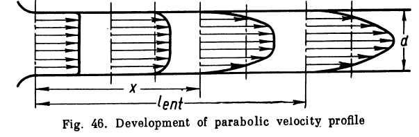
In the case of a straight pipe of uniform diameter leading from a reservoir, when the flow is laminar the velocity distribution at the entrance is practically uniform, especially if the entrance is rounded (Fig. 46). Further on viscous forces cause the velocity to change across a section: the layers in the vicinity of the wall are slowed down, but as the rate of discharge is constant for successive sections the velocity in the centre must be accelerated. More and more layers are gradually retarded until finally the parabolic velocity profile characteristic of laminar flow develops.

The section of a pipe from the entrance to the point where the pa­rabolic velocity profile develops is called the entrance, or transition, length (denoted l_eni). Beyond the entrance length steady laminar flow takes place and the velocity profile is parabolic as long as the pipe is straight and of same diameter. The laminar flow theory set forth here is valid only for steady laminar flow and cannot be applied to entrance conditions.

The entrance length can be determined from the following approx­imate formula in terms of the pipe diameter and Reynolds number:

(6.8)

Substituting Re_cr = 2,300 into Eq. (6.8), we obtain the maximum entrance length, which is 66.5 diameters.

As mentioned, resistance to flow in the entrance length is greater than in subsequent sections. The reason is that the value of the deriv­ative dvldy at the pipe wall in the entrance length is larger than in the steady-flow portions of the pipe. As a result, the shear stress, as determined by Newton's law, is greater, the more so the closer the considered section is to the pipe entrance, i.e., the smaller the coordinate x.

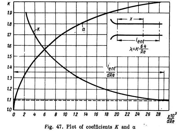
Loss of head in a pipe section, when l < l_ent is determined by Eqs (6.5) or (6.6) and (6.7), with a correction factor К greater than unity. The value of К can be found from the graph in Fig. 47, where it is given as a function of the dimensionless parameter . The greater the parameter the smaller К until, at

i. e., at x = l_ent, К = 1.09. Thus, the resistance of the entrance length of a pipe is 9 per cent higher than the resistance of an equal length with steady laminar flow.

For short pipes the factor K, as is apparent from the diagram, is substantially greater than unity.

When the length I of a pipe is greater than the entrance length l_enV the loss of head comprises the loss in the entrance length and the loss in the steady-flow portion, i. e.,

Taking into account Eqs (6.7) and (6.8) and after the necessary transformations and computations,

If the relative length of the pipeline -y is large enough, the num­ber 0.165 inside the parentheses can be neglected.. However, when

accurate calculations are necessary for pipelines whose length is commensurable with l_ent it must be taken into account.

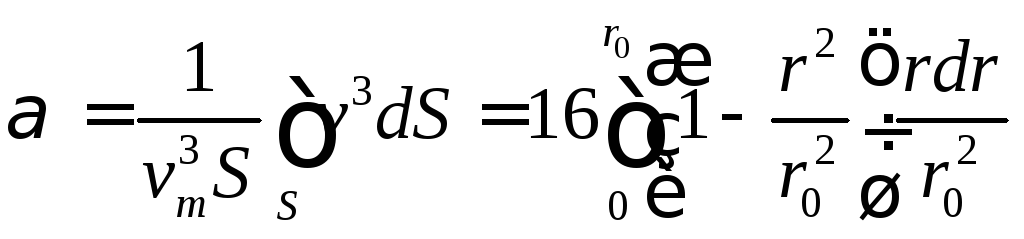
Knowing the velocity distribution law (6.1) and the relation be­tween mean velocity and loss of head (6.4) it is simple to determine the value of the coefficient a, which takes into account nonuniform velocity distribution when Bernoulli's equation is applied to steady laminar flow in circular pipes.

Take Eq. (4.15) and substitute into it the expressions (6.1) and (6.4) for the velocity and mean velocity, respectively. Then, taking into account that

and

dS = 2nrdr,

and after the necessary cancellations, we obtain

Substituting the variable

we obtain

(6.10)

Thus, the actual kinetic energy of a stream with laminar flow with parabolic velocity distribution is twice the kinetic energy of an iden­tical stream with uniform velocity distribution.

It can be demonstrated in like manner that the momentum of laminar flow with parabolic velocity distribution is P times greater than the momentum of a similar flow with uniform velocity dis­tribution, the coefficient (5 being constant:

For the transition length of a pipe with a rounded entrance the coefficient a increases from 1 to 2 (see Fig. 47).