

26. Turbulent flow in rough pipes
In
smooth pipes friction losses were completely determined by the
Reynolds number. In rough pipes, however, the value of Xt
depends
also on the roughness of the inside pipe surface. The important
point is not so much the absolute roughness size к
of
the projections
as the so-called relative roughness
![]() for the same absolute roughness
may have no effect on the resistance of a large pipe and
considerably
increase the resistance of a small one. Furthermore, the
shape and distribution of the projections may affect the resistance
of a pipe. The simplest case of roughness is that in which all the
projections are of the same shape and size, known as uniform
granular
wall roughness.
for the same absolute roughness
may have no effect on the resistance of a large pipe and
considerably
increase the resistance of a small one. Furthermore, the
shape and distribution of the projections may affect the resistance
of a pipe. The simplest case of roughness is that in which all the
projections are of the same shape and size, known as uniform
granular
wall roughness.
In
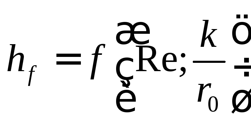
the case of uniform granular roughness the friction factor λt
depends
both on Re and on the ratio
![]() :
:
The effect of these two parameters on pipe friction is shown on the graph in Fig. 59, which is based on Nikuradse's experiments. Niku-radse investigated the resistance of artificially roughened pipes. He coated several different sizes of pipe with sand grains which had been segregated by sieving so as to obtain different sizes of grain of uniform diameter. In this way he obtained uniform granular roughness.
 The
pipes were tested in a broad range of relative roughnesses (
The
pipes were tested in a broad range of relative roughnesses (![]() = 1/500 to 1/15) and Reynolds numbers (Re = 500 to 106).
Fig.
59 contains the results of his experiments in the form of curves on
a logarithmic plot relating log (1,000 λ)
to
log Re for various ratios
= 1/500 to 1/15) and Reynolds numbers (Re = 500 to 106).
Fig.
59 contains the results of his experiments in the form of curves on
a logarithmic plot relating log (1,000 λ)
to
log Re for various ratios
![]() .
.
The inclined straight lines A and В correspond to the resistance laws for smooth pipes, i. e., Eqs (6.7) and (7.2), which, multiplied by 1,000 and the logarithm taken, give linear equations for the given coordinate system:
![]()
and
![]()
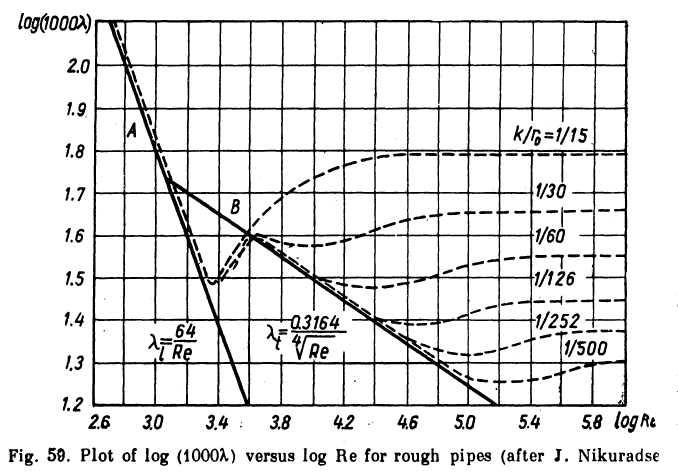
The broken lines are curves plotted for pipes with different relative roughness. The following basic conclusions can be drawn from the graph:
1. In laminar flow roughness does not affect resistance; the broke curves corresponding to various degrees of roughness practicall coincide with line A.
2. The critical Reynolds number practically does not depend on roughness. The broken curves diverge from line A at about the same value of Re.
3.
In
turbulent flow when Re and
![]() are small roughness does not affect
resistance; in some places the broken lines coincide with line B.
However,
with Re increasing the roughness begins to tell and the curves
for rough pipes begin to deviate from the straight line of the
resistance
law for smooth pipes.
are small roughness does not affect
resistance; in some places the broken lines coincide with line B.
However,
with Re increasing the roughness begins to tell and the curves
for rough pipes begin to deviate from the straight line of the
resistance
law for smooth pipes.
4.
At high values of Re and
![]() the friction factor kt
no
longer depends
on Re and becomes constant for a given relative roughness. This
corresponds to the horizontal portions of the broken lines after
their
slight rise.
the friction factor kt
no
longer depends
on Re and becomes constant for a given relative roughness. This
corresponds to the horizontal portions of the broken lines after
their
slight rise.
Thus,
for each of the curves corresponding to turbulent flow in rough
pipes there are observed three distinct regions of the numbers Re
and
![]() in which the behaviour of the friction factor λt
is
markedly
different:
in which the behaviour of the friction factor λt
is
markedly
different:
(1)
Low
Re and
![]() : λt
is
independent of the roughness and is controlled
solely by the Reynolds number, just as in smooth pipes. Roughness
has no maximum values.
: λt
is
independent of the roughness and is controlled
solely by the Reynolds number, just as in smooth pipes. Roughness
has no maximum values.
(2)
The
friction factor λt
depends
on both Re and
![]() .
.
(3)
High
Re and
![]() :
λt
is
independent of Re and is controlled solely
by the relative roughness; the resistance law is quadratic, as Xt
being
independent of Re makes head losses proportional precisely to the
square of the velocity [see Eq. (4.18)1; this is the "rough-law
regime".
:
λt
is
independent of Re and is controlled solely
by the relative roughness; the resistance law is quadratic, as Xt
being
independent of Re makes head losses proportional precisely to the
square of the velocity [see Eq. (4.18)1; this is the "rough-law
regime".
In order to gain a correct understanding of the resistance of rough pipes, it is,necessary to take into account the existence of the laminar sublayer mentioned in Sec. 25.
It was pointed out that with Re increasing the thickness of tha sublayer 6t decreases. For this reason in turbulent flow in a rough pipe with a low Reynolds number the laminar sublayer covers the projections, which are contained within it and do not affect the pipe resistance. As Re increases the thickness of the sublayer decreases and the projections extend partly outside it, thus beginning to affect the resistance. At large values of Re the sublayer practically vanishes and all the projections reach into the turbulent flow. Eddies form in the wake of each projection, which explains the quadratic resistance law in this regime.
Nikuradse carried out his experiments with artificially, uniformly granular-roughened pipes. For real rough pipes the dependence of λt on Re is somewhat different; notably there is no bulge in the curves following their divergence from the smooth-law curve. Fig. 60 presents a chart of some extremely precise experiments carried out by the Soviet scientist G. A. Murin.
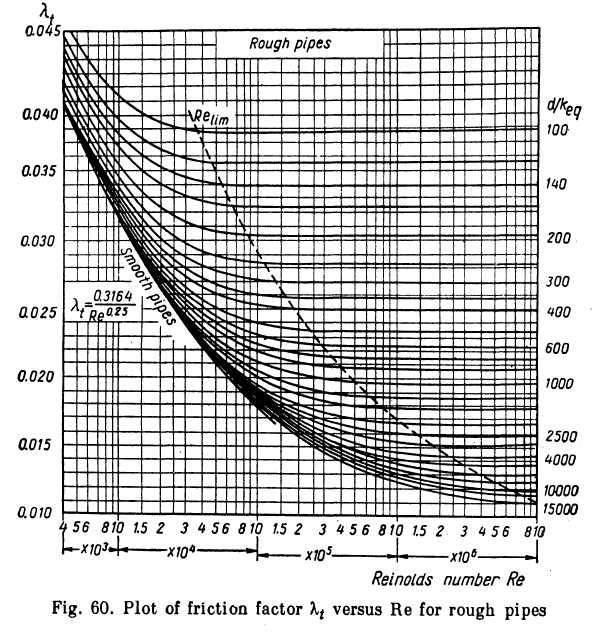
The
friction factor λt
for
real rough pipes is given as a function of Re
for different values of
![]() ,
where keq
is
the absolute roughness equivalent
to Nikuradse's granular roughness. For new steel pipes Murin
suggests assuming keq
=
0.06 mm, and for used pipes, keq
=
0.2
mm.
,
where keq
is
the absolute roughness equivalent
to Nikuradse's granular roughness. For new steel pipes Murin
suggests assuming keq
=
0.06 mm, and for used pipes, keq
=
0.2
mm.
The following new general formula has been suggested by the Soviet scientist A. D. Altshul for engineering calculations of the resistance of real rough pipes:
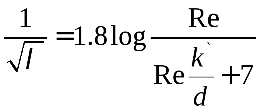 (7.4)
(7.4)
where d = pipe diameter;
k' = dimension proportional to absolute roughness. The limiting values of k' for different pipes are presented in Table 2.
Table 2
-
Pipe material
10³ k',mm
Glass tubing
Drawn tubing, brass, lead, copper
Seamless steel, high-grade manufacture
Steel pipe
Asphalt-dipped cast iron pipe
Cast iron pipe
0.0
0.0
0.6-2.0
3-10
10-25
25-50
At
low values of
![]() as
compared with the number 7, Eq. (7.4)turns
into Konakov's Eq. (7.1) for smooth pipes; at large values of
it turns into the equation for the rough-law regime (the quadratic
law of resistance):
as
compared with the number 7, Eq. (7.4)turns
into Konakov's Eq. (7.1) for smooth pipes; at large values of
it turns into the equation for the rough-law regime (the quadratic
law of resistance):
![]() (7.5)
(7.5)
Thus,
a comparison of the product
![]() with
the number 7 enables
a demarcation to be made between the different regimes of turbulent
flow through rough pipes.
with
the number 7 enables
a demarcation to be made between the different regimes of turbulent
flow through rough pipes.