

Chapter XI calculation of pipelines
43. Plain pipeline
We shall call a plain pipeline one of uniform diameter without branchings. The liquid flows along a pipe because its potential energy is higher at the initial point than at the terminal. This drop, or difference, in potential energy level can be produced by various means: difference in elevation, pumping or gas pressure.
In aeronautical engineering liquid flow in pipes is most commonly induced by pumps. In some liquid-propellant rocket systems and devices gas-pressure supply is employed. Liquid flow between different elevations, i. e., due to difference of elevation head, is employed only in ground conditions.
The principles of calculating pipelines set forth in this section (as well as in Sees 45 and 46) are equally applicable to all three methods of liquid supply, i. e., they do not depend on the method of producing the energy drop. The characteristic features of pumped flow are discussed in Sec. 47.
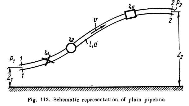
Let there be a plain pipeline of arbitrary geometry (Fig. 112) of total length / and diameter d with a number of local features in it. Suppose that at the initial section 1-1 the elevation head is z4 and the pressure* is pv and at the end section 2-2 the respective quantities are z2 and p2. Thanks to the uniformity of diameter (with the exception of the local features) the velocity v is uniform along the pipeline. Writing Bernoulli's equation between sections T-l and 2-2, assuming a, = a2 and cancelling out the velocity heads, we have,
![]()
or
![]()
We shall call the pressure-head difference in the left-hand side of the equation the required head Hreg; if the required head has been given in advance we shall call it the availableheadHnv. As is evident from the equation, this head comprises the geometrical elevation to which the liquid rises in its flow through the pipeline and the sum of all the head losses in the pipe. The latter can be represented in general form as an exponential function of the discharge. Then,
![]()
where the values of thecoefficient k and the exponent m vary depending on the flow regime.
For laminar flow, substituting the equivalent lengths for the local disturbances according to Eqs (6.5) and (8.19),
![]()
For turbulent flow, according to Eqs (4.17) and (4.18) and expressing the velocity in terms of discharge,
![]()
Equation (11.1), supplemented by the expressions (11.2) and (11.3), is the basic formula for calculating plain pipelines. It is also the pipeline characteristic equation.
A pipeline characteristic is a diagram on which the required head is plotted as a function of the rate of discharge of the pipeline. The larger the required discharge, the higher the required head. In lam inar flow the pipeline characteristic represents a straight (or nearly straight) line, in turbulent flow it is a parabola with an exponent of two (at λt = const) or about two (if the dependence of λt on Re is taken into account). The value of Δz is positive when the flow is from a lower to a higher elevation and negative when it is from a higher to a lower elevation.
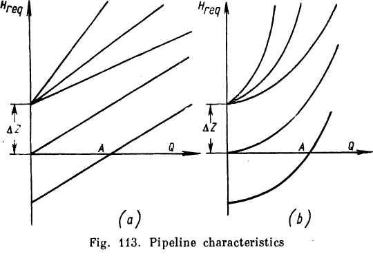
Pipeline characteristics are presented in Fig. 113 for the cases of (a) laminar and (b) turbulent flow. The slope of the curves depends on the coefficient k, increasing with the length of the pipeline increasing and the diameter decreasing and also with the minor losses increasing in the pipe. Besides, in laminar flow the slope of the curve varies as the viscosity of the liquid.
The intersection of the curve with the axis of abscissas (point A) gives the discharge for flow under gravity, i.e., only due to the elevation head difference Az. The required head in this case is zero as the pressure at both ends of the pipeline is atmospheric (taking the free surface in the higher reservoir as the beginning of the pipeline) (Fig. 114). If such a gravity pipeline empties into the atmosphere the velocity head must be added to the head losses in equation (11.1).
Let us examine some sample solutions of plain pipelines.
Problem 1. Given: discharge Q, fluid properties (y and v), pipeline dimensions, material and surface finish (roughness). To determine the required pressure Hreg
Solution.
First
determine the velocity of flow v
from
the rate of discharge and
pipe diameter d;
from
v
d and
v
determine Re and the flow regime; evaluate
the minor losses (![]() or
ζ in laminar flow and £ in turbulent flow) by the appropriate
formulas or experimentally; determine
X
according
to Re and the roughness;
finally, solve
or
ζ in laminar flow and £ in turbulent flow) by the appropriate
formulas or experimentally; determine
X
according
to Re and the roughness;
finally, solve 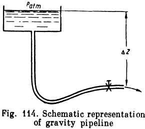 the
basic equation(11.1)
with respect to Hreg.
the
basic equation(11.1)
with respect to Hreg.
In laminar flow there is no need to compute X, and к can be determined directly from Eq. (11.2).
Problem 2. Given: available head Hav> fluid properties, pipeline dimensions and roughness. To determine the rate of discharge Q.
The solutions for laminar and turbulent flow differ markedly. The flow regime must therefore be assumed depending on the type (viscosity) of the liquid.*
For laminar flow, substituting the equivalent length for the minor losses, the solution is simple: from Eq. (11.1) and taking into account the expros- sion (11.2), determine the discharge Q, substituting Hqv for Hreq.
For turbulent flow the problem has to be solvea by trial and error or graphically.
In the first case we have one equation (11.1) with two unknown Quantities Q and Xt. To solve the problem a value is assigned to Kt according to tne roughness of the pipe. As Xt varies within fairly narrow limits (0.015 to 0.04), the error will not be very great, all the more so that in solving for Q Xt comes under the radical.
Solution of Eq. (11.1), taking into account (11.3), with respect to Q gives the rate of discharge to a first approximation. The obtained value of Q is used to determine v and Re to a first approximation, and from Re a closer value of A*. This new value of %* is substituted into the basic equation, which is solved again for Q. The secona approximation of the discharge will vary more or less from the first approximation. If the discrepancy is great, the procedure should be repeated until it is small enough. Usually two or three approximations are sufficient for the necessary accuracy.
For a graphical solution of the problem, the pipeline characteristic is plotted, taking into account the variability of %t% viz., a number of values are assigned to Q, and v, Re, kt and, finally, Hreq are computed from Eq. (11.1). By plotting Hreg against Q, and knowing the ordinate.//r^ = /irai;, the corresponding abscissa Q can be found.
Problem 3. Given: rate of discharge Q, available head Hatn fluid properties and all pipeline dimensions except diameter. To determine the diameter.
First a flow regime is assigned according to the fluid properties (v).**
* The flow regime can be determined by comparing Hav with its critical value Hcr Eqs (11.1) and (11.2) give
![]()
** The flow regime can be determined by comparing Hav with Hcn which, for a given Q, is
![]()
For
laminar flow the solution is simple. On the basis of (11.1), and
taking into
account (11.2),![]()
Having found d1 choose the nearest larger commercial diameter and, using the same equation, recalculate the value of the head for a given Q, or vice versa.
In turbulent flow, Eq. (11.1), taking into account (11.3), is best solved with respect to d in the following manner. Assign a number of standard values of d for a given Q and compute the corresponding values olHreg. Then plot a graph of # against d, and from the given H^ find the value ot d on the curve. Finally, choose the nearest larger commercial pipe diameter and solve again for Hreq.