Fundamentals of the Physics of Solids / 10-The Structure of Noncrystalline Solids

10.2 Quasiperiodic Structures		313
g(x + pλ) = g(x)	(10.2.14)

for all integers p. Because of the interaction between delocalized electrons and localized atoms the latter are expected to be displaced from their equilibrium positions, and the displacement to depend on the local electron density. Assuming a linear relationship, the new equilibrium position for the nth atom is

na + ug(na) ,

(10.2.15)

where the proportionality factor u that gives the modulation amplitude is determined by the interactions between electrons and atoms.

The density of atoms is given by

	∞
ρ(x) =		(10.2.16)
	δ[x − na − ug(na)].

n=−∞

When a beam is scattered by the system, the intensity of the di racted beam is determined by the absolute square of the structure amplitude

∞	∞
FK =	ρ(x)e−iKx dx = n=	−∞	e−iK[na+ug(na)]
−∞			(10.2.17)

∞

=e−iKnae−iKug(na)

n=−∞

defined in analogy to (8.1.27). If g(x) is a periodic function with period λ then so is exp[−iKug(x)], therefore it can be expanded into a Fourier series as

	∞
e−iKug(x) =
	ch(Ku)e2πihx/λ ,	(10.2.18)

h=−∞

hence	∞
∞
FK =	ch(Ku)e−ina(K−2πh/λ) .	(10.2.19)

n=−∞ h=−∞

Summation over n can be simplified exploiting (C.1.46) – that is, making use of the property that the sum over n is nonzero only if a(K − 2πh/λ) is an integral multiple of 2π:

∞∞

FK =	ch(Ku)δ[k − a(K/2π − h/λ)] .	(10.2.20)
	h=−∞ k=−∞

It is immediately seen that the structure factor is finite only for those values of K that can be written as

K =	2π	k +	2π	h .	(10.2.21)
	a		λ

314 10 The Structure of Noncrystalline Solids

Since h and k can take arbitrary integer values, besides the Bragg peaks associated with the lattice of periodicity a and the Bragg peaks due to the density variations of the electron system of periodicity λ, further peaks appear at all possible linear combinations of the two sets of reciprocal-lattice vectors. When λ a, these satellite peaks are close to the Bragg peaks of the original lattice. Although the examined system is one-dimensional, di raction peaks are specified by two integers. Owing to the incommensurability of the two wavelengths the allowed Ks are dense all along the line. Nevertheless the di raction pattern is a set of relatively well separated sharp peaks (sharp dots on a film) as amplitude is usually large only for reflections with a low index. This is well illustrated by the choice g(x) = sin x. Using (C.1.50) it can be shown that the expansion coe cients appearing in (10.2.20) are the Bessel functions, which are known to decrease fairly rapidly with increasing orders.

Similar conclusions apply to the case when atomic positions in a threedimensional lattice are subject to modulation with an incommensurate periodicity. Let the position of the jth atom in the nth primitive cell be denoted by

r(n, j) = Rn + rj + uj sin[q · (Rn + rj ) + ϕj ] .

(10.2.22)

If the scattering amplitude of the jth atom of the primitive cell is fj , the structure amplitude is

FK =	fj e−iK·r(n,j)
n,j	(10.2.23)
=	fj e−iK·(Rn +rj )e−iK·uj sin[q·(Rn+rj )+ϕj ] .
n,j

The second exponential term can again be expanded into a series of Bessel functions,

	∞
FK =	(−1)mfj e−i(K−mq)·(Rn +rj )eimϕj Jm(K · uj ) . (10.2.24)
	n,j m=−∞

Summation over the vectors Rn labeling the primitive cells yields finite contributions only when K − mq is a vector of the reciprocal lattice – that is, di raction peaks are found in directions for which

K = hb1 + kb2 + lb3 + mq .

(10.2.25)

Di raction peaks are now specified by four integers.

10.2.3 Experimental Observation of Quasicrystals

We saw in Chapter 6 on the symmetries of crystalline structures that translational symmetry allows only two-, three-, four-, and sixfold rotation axes. It was also asserted that fivefold symmetry is ruled out because the plane cannot

10.2 Quasiperiodic Structures

315

be tiled perfectly with regular pentagons. When discussing the Laue method of structural analysis in Section 8.2.3 it was mentioned that the Laue pattern had to possesses the same rotational symmetries as the crystal itself around the direction of the incident beam.

In the light of these not without reason did the discovery of D. Shechtman, I. Blech, D. Gratias, and J. W. Cahn made in 1984 cause great sensation. When studying a quenched sample of an aluminum-manganese alloy (Al86Mn14) using electron di raction methods it was noticed that, depending on the direction of observation, the Laue patterns exhibited symmetries characteristic of two-, threeand fivefold rotational axes, as if the crystal possessed icosahedral symmetry. Such di raction patterns are shown in Fig. 10.6.

Fig. 10.6. Two-, three-, and fivefold symmetry in the electron di raction patterns of quasicrystalline Al86Mn14 [D. Shechtman et al., Phys. Rev. Lett. 53, 1951 (1984)]

Soon a broad class of materials that exhibit similar features was discovered: their di raction patterns show symmetries that cannot be interpreted within the framework of traditional crystallography. In addition to the abovementioned Al86Mn14, icosahedral symmetry is observed in Al86Fe14, Al85Cr15, and Al65Cu20M15 (where M stands for Mn, Fe, Cr, V, Ru, or Os). The appearance of icosahedral regions in quenched transition-metal alloys is in fact not surprising. For spherical atoms in a crystalline environment the closest packing is known to be o ered by fcc and hcp structures of coordination twelve. For transition metals, where d orbitals play an important role, the energetically most favorable arrangement in a cluster of 13 atoms does not correspond to the local environment in fcc or hcp structures (cuboctahedra or anticuboctahedra): here the twelve nearest neighbors are arranged icosahedrally around the thirteenth, as shown in Fig. 7.9. In the new class of materials the building blocks are such icosahedral units, however their positions show no long-range order. Nevertheless some kind of long-range order, namely bond-orientational order is preserved. Although discrete translational symmetry is broken, the structure is quasiperiodic under translations. Such materials are called quasicrystals, abbreviated from quasiperiodic crystals.

316 10 The Structure of Noncrystalline Solids

In addition to icosahedral symmetry, other symmetries ruled out in conventional crystallography may also appear in quasicrystals. Eight-, tenand twelvefold symmetries are observed in Mn82Si15Al3, Al65Cu20Mn15, and V15Ni10Si, respectively. Needless to say, there are many other examples for each case. Quasicrystals can be classified according to their noncrystallographic symmetries, thus we speak of octagonal, decagonal, dodecagonal, and icosahedral quasicrystals.

The absence of long-range periodic order in atomic positions is clearly shown by the partial distribution functions in Fig. 10.7. While oscillations are damped less rapidly than in amorphous materials, the radial distribution function is nevertheless closer to that of amorphous materials than of crystals. On the other hand the di raction pattern indicates the presence of a longrange quasiperiodic order – just like in incommensurate structures. Contrary to the latter, where only crystallographically allowed rotations are observed, quasicrystals show rotational symmetries that are ruled out in 3D crystals. In fact quasiperiodicity is precisely due to such symmetries; even the shape of quasicrystals may reflect these symmetries.

g(r)

4

2	Al Al

0

-2

Al Mn

-4

Mn Mn

-6

-8

-10			8
2	4	6		10	12	14

r (Å)

Fig. 10.7. Partial distribution functions for Al–Al, Al–Mn, and Mn–Mn in icosahedral quasicrystalline Al74Si5Mn21, measured by M. de Boissieu et al. (J. Phys.: Condens. Matter 2, 2499 (1990)) using neutron di raction techniques. For better visibility, curves are shifted vertically

Without going into mathematical details, we shall now sketch a simple model for quasicrystalline order that also explains the appearance of relatively sharp Bragg peaks.

10.2 Quasiperiodic Structures

317

10.2.4 The Fibonacci Chain

We shall start the analysis of the di raction patterns of quasicrystals with the example of a one-dimensional quasiperiodic arrangement, a chain built up of short (S) and long (L) segments according to the construction rule of the Fibonacci sequence.2 The zeroth generation of the Fibonacci sequence consists of a single element S, and the first generation is composed of a single element L. Then, starting from the second generation, the nth generation is obtained by joining the two previous ones. The Fibonacci sequences constructed in this way using the Fibonacci rule Σn = Σn−1 + Σn−2 are shown in Table 10.1.

Table 10.1. Construction of new generations of Fibonacci sequences by joining the two previous ones. The number of elements in the sequence is always a Fibonacci number

Fibonacci number	Fibonacci sequence
1	S
1	L
2	LS
3	LSL
5	LSLLS
8	LSLLSLSL
13	LSLLSLSLLSLLS
21	LSLLSLSLLSLLSLSLLSLSL
34	LSLLSLSLLSLLSLSLLSLSLLSLLSLSLLSLLS

Note that the nth generation of the sequence can be obtained from the (n − 1)st generation by replacing each S by an L (S → L), and each L by an L and S (L → LS). When L and S are identified as long and short segments

placed along a line, and the ratio of the lengths of the two segments is the

√

golden mean τ = (1 + 5)/2 = 1.618 . . . , then the chain generated with the above method is called the Fibonacci chain. The Fibonacci chain has the interesting feature that if the lengths of the segments are scaled down by τ in every iteration step, the overall length of the chain is left unchanged because of the relation

	1	1 +	1	= 1 .	(10.2.26)
	τ		τ

Figure 10.8 shows the result of two successive iteration steps.

Now consider identical atoms placed along a line, separated by short and long distances according to the sequence in the Fibonacci chain. When di raction is performed as a thought experiment, the resulting pattern is easily determined numerically, since according to Eq. (8.1.50) the amplitude is given

2 Leonardo Pisano (Leonard of Pisa), commonly known as Fibonacci, 1202.

318

10 The Structure of Noncrystalline Solids

L

S

L

L

S

L

S

L

L

S

L

L

S

L

S

L

L

S

L

L

S

L S L L S L S L L S L L S L S L L S L S

L

Fig. 10.8. Equal-length Fibonacci chains obtained using the rules L → (L + S)/τ and S → L/τ

by the Fourier transform of the distribution of atoms. Because of the lack of periodicity, the Fourier components are densely distributed. Nevertheless, as shown in Fig. 10.9, sharp peaks are observed in the di raction pattern; their positions can be specified by two indices, as expected for a one-dimensional quasiperiodic system.

Intensity

																																					3,2)																			(5,3)
																																					(
																																					(2,1)
																															(1,1)							)
																												(0,1) (1,0)					(2,0) (1,2)					(2,2 3,1)												(4,2)
																																									(
10														5								0															5													10								K

Fig. 10.9. Numerically determined di raction pattern (Fourier spectrum) of a finite Fibonacci chain. The scale of K corresponds to 1/S. The peaks are labeled with two integers, as explained in the text [R. D. Diehl et al., J. Phys.: Condens. Matter 15, R63 (2003)]

Choosing the position of the (1, 0) peak as unity, the (0, 1) peak is found at 1/τ , and the peak with indices (h, k) at h + k/τ . Note that there is some arbitrariness in indexing. Since the ratio of the two elementary lengths – the positions of the peaks (1, 0) and (0, 1) – is just τ , it follows from (10.2.26) that another consistent indexing is obtained by choosing the unity τ times larger or smaller. In the latter case the new indices h and k are related to the old ones by h = h + k and k = h. This indicates the absence of a natural length scale in the Fibonacci chain – and quasicrystals in general. Note that whichever indexing is chosen, the intensity will be large for those peaks in which the two indices are subsequent Fibonacci numbers.

To demonstrate this, we shall calculate analytically the Fourier components that correspond to the quasiperiodic spectrum, and from them the

10.2 Quasiperiodic Structures

319

di raction pattern. To this end we shall make use of another construction of the Fibonacci sequence. Consider the sequence of numbers m/τ , wherex (“floor x”) denotes the integer part of x, i.e., the largest integer less than or equal to x. Starting with m = 1, we have

m/τ = 0, 1, 1, 2, 3, 3, 4, 4, 5, 6, 6, 7, 8, 8, 9, 9, 10, . . ..

Now taking the di erence between adjacent numbers,

34

m + 1		−	5	m	6	= 1, 0, 1, 1, 0, 1, 0, 1, 1, 0, 1, 1, 0, 1, 0, 1, . . . .	(10.2.27)
τ				τ

When each 1 is replaced by L and each 0 by S, the Fibonacci chain is recovered. Thus a mathematical formula can be given for the alternation of long and short segments. The mth place is occupied by a long (L) segment if

34

m + 1		=	5	m	6	+ 1 .	(10.2.28)
τ				τ

On the other hand, if

34

m + 1	=	5	m	6	,	(10.2.29)
τ			τ

then there is a short (S) segment in the mth place. Consequently, expressed in units of the length of the shorter segment, the distance of the mth point of the Fibonacci chain from the origin is

xm = S m + (τ − 1) 3			τ	4 = S m + τ	3	τ	4 .	(10.2.30)
			m + 1	1		m + 1
Using the Heaviside step function this can be alternatively written as
xm = S m +	n	(τ − 1)nθ n + 1 − (m + 1)/τ θ (m + 1)/τ − n						. (10.2.31)

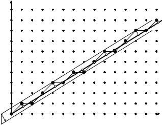
This result is simply illustrated, and the illustration is easily generalized to the description of quasicrystals in higher dimensions. Consider a two-dimensional square lattice of lattice constant a, and mark the points (m, n) for which n = (m+1)/τ . Then these points are projected onto the straight line of slope tan φ = 1/τ . This is shown in Figure 10.10. It is clear from the construction that the distance of the mth point from the origin is

xm = a m cos φ + a (m + 1)/τ sin φ .

(10.2.32)

When the lattice constant is chosen as a = S/ cos φ, these distances are the same as in (10.2.30), so this construction generates a Fibonacci chain, too.

When adjacent points (m, n) in the figure are connected, long (short) segments of the Fibonacci chain are seen to be the projections of diagonal (horizontal) edges of a square cell in the lattice. Note that the selected lattice

320 10 The Structure of Noncrystalline Solids

	y
l	x

Fig. 10.10. Construction of the Fibonacci chain via the projection of selected points of a two-dimensional square lattice

points are inside a strip of width l = a cos φ around the line of slope 1/τ , and the above-defined trajectory passes through all lattice points within the strip. This implies that the quasiperiodic Fibonacci chain can also be constructed by projecting the points inside a finite strip of the square lattice on a straight line with an irrational slope of 1/τ .

Yet another, frequently used representation of the Fibonacci chain is obtained by adding to the previously selected set of lattice points the corner points below the long diagonal sections – i.e., for every m those points (m, n) are chosen for which n = m/τ or n = (m + 1)/τ , and then these points, which form a quasiperiodic staircase, are projected on the line with slope tan φ = 1/τ , as shown in Fig. 10.11. Compared to the previous staircase that was obtained by connecting the points (m, n), horizontal sections are preserved, while each diagonal section is replaced by a horizontal plus a vertical one. It follows from the scaling property of the Fibonacci chain that the projected points once again form a Fibonacci chain – however, now the projections of horizontal edges are long segments and those of vertical edges are short segments. The length of the latter is, of course, 1/τ times the former, that is, S = a sin φ. This construction corresponds to the following algorithm. Elements of the Fibonacci chain are chosen in succession; for long elements (L) a step is made to the right on the square lattice, for short ones (S) a step is made upward. The staircase traced out in the two-dimensional lattice lies in a strip whose slope is tan φ = 1/τ and whose width l is the projection of

the unit square on the direction perpendicular to the strip, i.e.,
l = a(cos φ + sin φ) = S(τ + 1) = Sτ 2 .	(10.2.33)

10.2 Quasiperiodic Structures

321

y

x

Fig. 10.11. Another construction of the Fibonacci chain via the projection of selected points of a two-dimensional square lattice

To evaluate the amplitude of the scattered beam consider the di raction by a system that contains the points of a planar square lattice within a strip of finite width. For simplicity, we shall present the calculation in the model that represents the Fibonacci chain by the projections of points (m, (m + 1)/τ ). Using formula (10.2.31) for the coordinates,

e−iKxm = e−iKS(m+n/τ )θ n + 1 − (m + 1)/τ θ (m + 1)/τ − n .

mm,n

(10.2.34) When the two-dimensional vector K ≡ (Kx, Ky) = (K, K/τ ) is introduced, the previous expression can be written as

m e−iKxm =	dr e−iK·r m,n δ(x − Sm)δ(y − Sn)	(10.2.35)

×θ[y/S + 1 − (x/S + 1)/τ ]θ[(x/S + 1)/τ − y/S] .

Next, the function to be Fourier transformed is considered as a product of two terms; the first contains a summation over all points of the square lattice, and the second is a product of step functions projecting them to the narrow strip. Their respective Fourier transforms are easily determined,

dr e−iK·r δ(x − Sm)δ(y − Sn)

m,n

(10.2.36)

= NV (2π)2 δ(Kx − h2π/S)δ(Ky − k2π/S) ,

h,k

322 10 The Structure of Noncrystalline Solids

and

dr e−iK·r θ[y/S + 1 − (x/S + 1)/τ ]θ[(x/S + 1)/τ − y/S]

	(x+S)/τ
=	dx		dy e−iK·r	(10.2.37)
=	(x−S/τ )/τ		e−iKy (x+S)/τ − e−iKy (x−S/τ )/τ .
	dx e−iKx x Ky
		i

Since the Fourier transform of the product is the convolution of the Fourier transforms of its factors,

m	e−iKxm = (2π)2	V	h,k	dx	dqxdqy δ(Kx − qx − h2π/S)			(10.2.38)
		N
	×δ(Ky − qy − k2π/S)e−iqxx					i	e−iqy (x+S)/τ − e−iqy (x−S/τ )/τ .
						qy
Integration yields a factor
		δ[K(1 + 1/τ 2) − (2π/S)(h + k/τ )] ,						(10.2.39)

indicating that di raction peaks appear for those values of K that satisfy

2π τ 2

2π

1

K = Khk =

(h + k/τ ) =

√

(hτ + k) ,

(10.2.40)

S

1 + τ 2

a

1 + τ

2

where h and k are integers. Writing the structure amplitude as

FK =

Fhk δ(K − Khk) ,

(10.2.41)

hk

the Fourier coe cient is found to be

Fhk =

=

1
lim		e−iKxn
N →∞ N		n

πτ

sin 1 + τ 2 (τ k − h)

πτ

1 + τ 2 (τ k − h)

(10.2.42)

		τ + 2		−
exp	iπ	τ − 2	(τ k		h) .

Thus di raction peaks are indeed specified by two integer labels. The intensity of the di raction peak of indices hk is found to be proportional to

sin2		1 + τ 2 (−h + τ k) .	(10.2.43)
		πτ

		2
	1 + τ 2 (−h + τ k)
	πτ