2.7. Analysis of accounts receivable

In the national financial and economic literature, much attention is paid to analysis of the structure of current assets to the achievement of their equilibrium, to the identification of reserves for reduction accounts receivable, to rationalization of cash flows and inventory. However, in publications of scientific and educational nature there are insufficiently represented the theoretical and methodological approaches, based on systematic research into the causes and consequences of company's debtors for its products shipped and services rendered. In essence it comes to building management system of accounts receivable which would control the relationships with debtors and would regulate the size of debt within the limits that provide liquidity and financial security.

G. Chitaya⁷ offers a method of constructing a system of management of accounts receivable, including a statistical analysis of the effectiveness of the actual level of management and use of company's human resources capacity without the formation of a specialized organizational structure. The aim is to demonstrate the approach to improving working capital management on the basis of designing an effective system of enforcement, reduction and control of receivables.

Statistical analysis of the effectiveness of company's accounts receivable

Based on of data of company's receivables by major debtors there can be evaluated the effectiveness of management using the methods of statistical analysis of variations. These, above all, are such indicators as the weighted arithmetic mean, mode, median, concentration ratio and the uneven distribution of attribute (accounts receivable). In the latter case it comes to the legitimacy of using the Gini coefficient, Herfindahl, variations, as well as graphic illustrations of uneven distribution of debtors using the Lorenz curve.

Obtaining analytical statistical tables, which allows to determine the characteristics of the of the variation series of accounts receivable of the enterprise involves a series computational actions.

1. Determining the optimal number of groups for the collection of debtors.

At this stage, application of Sturges formula is appropriate:

r = 1 + 3,32 lg n = 1 + 1,44 ln n, (2.7.1)

where n - number of population units (enterprises-debtors).

Since n = 45 (the number of debtors, according to Appendix 1)

r = 1 + 1.44 ln n = 1 + 1.44 ln (44) ≈ 6.45, number of groups can be taken as 6, i.e. r = 6.

Establishment of interval variational series of debtors

Intervals are set regarding to concentration of accounts receivable (see column A, table 2.7.1)

Table 2.7.1. The calculation of basic statistical characteristics of variational series of accounts receivable of the enterprise by major debtors

Accounts receivable, thousand rur			Number of debtors			Interval mean, xi		ximi		Cumulative frequencies Fi		Relative cumulative frequencies Pi, %		Distribution density, %,		Proportion of acc. rec. of groups of debtors in total
														Yk = wi /
xk – 1	xk	mi		in % to total, wi									/ xk				Cumulative, qi
А	B	1		2	3		4		5		6		7		8		9	10		11
0	10	14		31,1	5		70		14		31,1		3,11		0,0010		0,0010	0,000001		350,00
10	100	6		13,3	55		330		20		44,4		0,15		0,0046		0,0056	0,000022		18 150,00
100	500	12		26,7	300		3600		32		71,1		0,07		0,0507		0,0563	0,002571		1 080 000,00
500	1 000	4		8,9	750		3000		36		80,0		0,02		0,0423		0,0986	0,001785		2 250 000,00
1 000	10 000	8		17,8	5500		44000		44		97,8		0,0020		0,6197		0,7183	0,384051		242 000 000,00
10 000	30 000	1		2,2	20000		20000		45		100,0		0,0001		0,2817		1,0000	0,079349		400 000 000,00
	Total	45		100			71000								1			0,46778		645 348 511,00

The calculation of the average characteristics of interval variations of the series: a weighted average, mode and median

The weighted average will be:

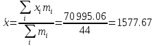(2.7.2)

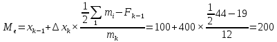
Mode (Mo) for a series with unequal intervals is determined using a density distribution of (Yk). This is feature value that occurs most often in units of the aggregate. For a discrete series mode will be the option with the greatest frequency

Distribution density is the highest in group 1:

Yk = Y1 = 2,96.

(2.6.3)

Median (Me) is a feature value falling in the middle of a ranked set (for ranged series with an odd number of individual values ​​of the median would be the value, which is located in the center of the series, in this case 44 / 2 = 22), is calculated using the cumulative frequency index:

(2.7.4)

The same value is obtained if we use the cumulative relative frequency.

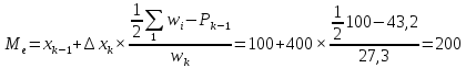(2.7.5)

Calculation of variation

Dispersion (D):

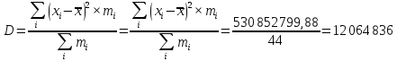(2.7.6)

Standard deviation:

(2.7.7)

Coefficient of variation:

(2.7.8)

Calculation of the Gini concentration coefficient (G)

This ratio is used to measure the degree of uneven distribution of population units (accounts receivable of the company in 2009). This ratio it is appropriate to define by formula:

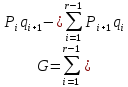(2.7.9)

where Pi and Pi + 1 are consecutive values of the accumulated relative frequencies;

qi and qi + 1 are consecutive values ​​of the elements of column 9 table 1;

qi (i =) are calculated according to the cumulative elements of column 8 table 1.

The results of support the calculations required to obtain the value of the Gini coefficient are given in Table 2.7.2.

(2.7.10)

Table 2.7.2. Intermediate estimates for the Gini coefficient of uneven distribution of accounts receivable of the company

Piqi+1		Pi+1qi+
29,5*0,0056=	0,164411076	43,2*0,0009=	0,039575
43,2*0,0563=	2,429945947	7,05*0,0056=	0,392057
70,5*0,0985=	6,941808209	79,5*0,0563=	4,476216
79,5*0,7183=	57,13672669	97,7*0,0985=	9,62896
97,7*1=	97,72727273	100*0,7183=	71,82903
Total:	164,4001646	Total:	86,36584

Establishing Herfindahl coefficient

This ratio indicates the total proportion of the dominant group among the debtors of the company (H) and is calculated as follows:

(2.7.11)

In accordance with data in table 2.7.1. H (%) = 46,78%

The calculation of the asymmetry coefficient of Pearson (K_as)

(2.7.12)

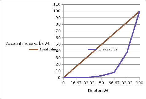
Using the Table. 2, there can be constructed Lorentz curve. On a horizontal axis there will be located cumulative relative frequency (Pi), and on a vertical there will be values of the parameters qi. Coordinates of the points the diagonal line correspond to equal values ​​of the pair (Pi, qi). They are increasing multiple of 100 / 6 = 16.67.

Lorenz curve of uneven distribution of accounts receivable of analyzed company in 2009 is shown in Fig. 2.7.1.

Figure 2.7.1. Lorenz curve of accounts receivable distribution for 2009

Statistical indicators for assessing the distribution of enterprise's debtors by value of their debt may be used to assess the effectiveness of current assets management, and above all, their most significant part - accounts receivable. Table 2.7.3 represents the main statistical indicators of efficiency assessment for accounts receivable management.

Table 2.7.3. Main statistical indicators of efficiency assessment for accounts receivable management for 2009

Indicator	Symbol	Value
Weighted average, thousand rur.	x	1 577,67
Mode, thousand rur.	Мо	1,743
Median thousand rur.	Ме	200
Variance	D	11 064 836
Standard deviation, mln rur.	s	3473,45
The coefficient variation,%	n	220,16
The Gini coefficient,%	G	0,78
Herfindahl coefficient,%	H	46,78
The asymmetry coefficient of Pearson	Кas	0,45

Weighted arithmetic average of accounts receivable was 1,613.64 rubles. For 44 debtors the value is small that is a consequence of the greater concentration of debt up to 1 million rur. This is evidenced by values of mode and median (1.743 and 200 thousand rubles., respectively). According to the value of Pearson coefficient, the asymmetry of the total debt debtors is dextral. From the general theory of statistics it is known that if the ratio , where and n is the number of debtors, then the asymmetry of distribution is reasonable, despite the heterogeneity of total debts. In given case, this ratio is 1.31 and indicates a moderate asymmetry of the aggregate. This is confirmed by the fact that the median is located between mode and a weighted average. It follows that the distribution of the receivables can be explained within the framework normal probability law, which, in turn, allows assessing the degree of predictability of debtors that is their controllability. The high value of standard deviation (3473.45 thousand rub.) indicates a large scatter in accounts receivable and indicates the existence of risk in dealing with collection of its expired parts.

The high level of variation coefficient characterizes the inhomogeneity of total receivables and a low degree of controllability. The Gini coefficient shows that the distribution of accounts receivable is uneven (78%) and most of the debt is concentrated in the dominant group, accounting for 46.78% (Herfindahl coefficient).

Identified patterns using statistical methods to a large extent demonstrate the risks and low accounts receivable management effectiveness and the feasibility of designing an improved system.