

Measurement and Control Basics 3rd Edition (complete book)
.pdfChapter 10 – Final Control Elements |
285 |
tain physical conditions. You must therefore take them into account when selecting the proper valve for a given application.
Flashing and Cavitation
Flashing and cavitation involve a change in the form of the fluid media from the liquid to the vapor state. The change is caused by an increase in fluid velocity at or just downstream of the flow restriction, normally at the valve port or inside the body.
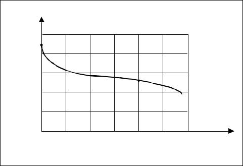
To simplify our discussion of flashing and cavitation, let’s imagine process in which there is a simple restriction in the line. As the flow passes through the physical restriction, there is a necking down, or contraction, of the flow stream. The point at which the cross-sectional area of the flow stream is smallest is called the vena contracta, which is just a short distance downstream of the physical restriction (Figure 10-6).
|
Restriction |
|
|
|
Vena Contracta |
|
|
|
|
|
|
|
|
|
|
|
|
|
|
|
|
|
|
|
|
|
|
|
|
|
|
|
|
|
|
|
|
|
|
|
|
|
|
|
|
|
|
Flow
Pin 


 Pressure loss
 P
P
Plow
Low pressure at Vena Contracta
Figure 10-6. Illustration of vena contracta
To understand flashing and cavitation, you first need to understand the interchange between the kinetic and potential energy of a fluid flowing through a valve or other restriction. To maintain a steady flow of liquid through the valve, the velocity must be greatest at the vena contracta. This increase in velocity, or kinetic energy, comes about at the expense of pressure, or potential energy. The pressure profile along the valve shows a sharp decrease in pressure as velocity increases. The lowest pressure, of course, will occur at the vena contracta, where the velocity is the greatest. Then, farther downstream, as the fluid stream expands into a larger area, velocity will decrease and thus pressure will increase. The pressure down-
286 Measurement and Control Basics
stream of the valve never recovers completely to the level that existed upstream.
The pressure differential that exists across the valve is called the ∆P of the valve. This ∆P is a measure of the amount of energy that was dissipated in the valve. Useful energy is lost in the valve because of turbulence and friction. The more energy is dissipated in a valve, the greater the ∆P for a given area and flow.
If two valves have the same flow area and upstream pressure and are passing the same flow, then it follows that they must have the same velocities at the vena contracta. This, in turn, means that the pressure drop from the inlet to the vena contracta must also be the same. On the other hand, if one valve dissipates less energy due to turbulence and friction, more energy will be left over for recovery in the form of downstream pressure. Such a valve would be relatively streamlined and classified as a high-recovery valve. In contrast, a low-recovery valve dissipates more energy and, consequently, has a greater ∆P for the same flow.
Regardless of the valve’s recovery characteristics, the amount of liquid flow is determined by both the flow area and the flow velocity. If the flow area is constant, such as when the valve is wide open, then any increase in flow must come from an increase in fluid velocity. An increase in velocity results in a lower pressure at the vena contracta. This logic leads to the conclusion that the pressure differential between the inlet and the vena contracta is directly related to the flow rate. The higher the flow rate, the greater is the pressure differential across the control valve.
If the flow through the valve increases, the velocity at the vena contracta must increase, and the pressure at that point will decrease accordingly. If the pressure at the vena contracta should drop below the vapor pressure for the liquid, bubbles will form in the fluid stream. The rate at which bubbles form will increase greatly as the pressure is lowered further below the vapor pressure. At this stage of development, there is no difference between flashing and cavitation. It is what happens downstream of the vena contracta that makes the difference.
If the pressure at the outlet of the valve is still below the vapor pressure of the liquid, the bubbles will remain in the downstream system creating what is known as flashing. If the downstream pressure recovery is sufficient to raise the outlet pressure above the liquid vapor pressure, the bubbles will collapse, or implode, producing cavitation. It is easy to visualize why high-recovery valves tend to be more susceptible to cavitation since the downstream pressure is more likely to rise above the vapor pressure.
Chapter 10 – Final Control Elements |
287 |
The implosion of the vapor bubbles during cavitation releases energy that manifests itself as noise and physical damage to the valve. Millions of tiny bubbles imploding nearby the valve’s solid surfaces can gradually wear away the material, causing serious damage to the valve body or its internal parts. It is usually quite apparent when a valve is cavitating; a noise much like gravel flowing through the valve will be audible. Areas damaged by cavitation also appear rough, dull, and cinder like.
Flashing can also damage valves, but it will produce areas that appear smooth and polished since flashing damage is essentially erosion. The greatest flashing damage tends to occur at the point of highest velocity.
Choked Flow
The noise and physical damage to the valve that cavitation and flashing cause are important considerations when sizing a valve, but even more important is that they limit flow through the valve. During both phenomena, bubbles begin to form in the flow stream when the pressure drops below the vapor pressure of the liquid.
These vapor bubbles cause a crowding condition at the vena contracta that reduces the amount of liquid mass that can be forced through the valve. Eventually, the flow is saturated or choked and can no longer be increased.
The valve-sizing equation (Equation 10-10) implies that there is no limit to the flow you can obtain as long as the ∆P across the valve increases. However, this is not true if flashing or cavitation occur. Assuming that the upstream pressure is constant, the flow that can be achieved by decreasing the downstream pressure is limited.
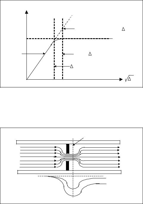
The flow curve deviates from the relationship predicted by the basic liq- uid-sizing equation (Equation 10-11) because of the vapor bubbles that appear in the flow stream during flashing or cavitation. If you increase the valve pressure slightly beyond the point where bubbles begin to form, the flow will become choked. Assuming constant upstream pressure, a further increase in ∆P will not increase the flow. This limiting pressure differential is called “∆P allowable” or ∆Pa. Figure 10-7 shows how the ∆Pa is related to the basic liquid-sizing equation and the choked flow. Equation 10-11 will plot as a straight line if the horizontal axis is the square root of ∆P, with a slope equal to the valve-sizing coefficient (Cv). If you use the actual service ∆P in the basic liquid-sizing equation when ∆P > ∆Pa, the equation will predict a much larger flow than will actually exist in service.
The choked flow is the flow that will actually exist in service when ∆P is greater than ∆Pa. These two conditions are illustrated in Figure 10-8. The
Chapter 10 – Final Control Elements |
289 |
can vary widely from one style of valve to the next, it is quite predictable for any given valve and you can easily determine it by test. The experimental coefficient that is used to define the point of choked flow for any valve is called Km.
For a given flow, the pressure drop across the valve is a measure of the valve-recovery characteristics. At the point of choked flow, the pressure drop is ∆Pa. We showed earlier that the pressure differential from the inlet to the vena contracta is a measure of the amount of flow being forced through the valve. The ratio of these two pressure differentials, when the valve has just reached choked flow, is defined as the valverecovery coefficient (Km):
|
Km = |
∆ Pa |
|
(10-12) |
|
P1 − Pvc |
|||
|
|
|
||
where |
|
|
|
|
P1 |
= inlet pressure (psia) |
|
||
Pvc |
= vena contracta pressure at the point of choked flow (psia) |
|||
∆Pa |
= the allowable differential pressure across the valve |
|
||
With constant upstream pressure, ∆Pa is the maximum pressure drop across the valve that will effectively increase the flow. From this definition, you can see that Km relates the valve’s pressure-recovery characteristics to the amount of flow passing through the valve.
Consider two valves that are passing the same choked flow but have different recovery characteristics. One is a high-recovery valve and the other is low-recovery. Figure 10-8 shows the pressure profiles for two such valves. Since both valves have just reached the same choked flow, the pressure differential from the inlet to the vena contracta is the same for both of them. On the other hand, the pressure-recovery characteristics, and consequently the ∆Pa values, are significantly different. Relating this to the definition of Km, it is easy to see that the high-recovery valve will have a much smaller Km value than the lowrecovery valve.
In effect, Km describes the relative pressure-recovery characteristics of a valve. High-recovery valves will tend to have low Km values, and lowrecovery valves will tend to have higher Km values. A typical range of Km values is from about 0.3 to 0.9. The values for valves with intermediaterecovery characteristics will be somewhere within this range.
Equation 10-13 shows the Km expression rearranged into a more useful form:
∆ Pa= Km (P1− Pvc ) |
(10-13) |
Chapter 10 – Final Control Elements |
291 |
|
1.0 |
|
|
|
|
|
c |
|
|
|
|
|
|
- r |
0.9 |
|
|
|
|
|
Ratio |
|
|
|
|
|
|
|
|
|
|
|
|
|
Pressure |
0.8 |
|
|
|
|
|
0.7 |
|
|
|
|
|
|
Critical |
|
|
|
|
|
|
0.6 |
|
|
|
|
|
|
|
0.5 |
|
|
|
|
|
|
0 |
.20 |
.40 |
.60 |
.80 |
1.00 |
Vapor Pressure (PSIA)
Critical Pressure (PSIA)
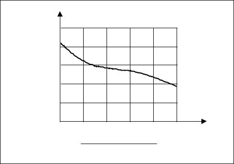
Figure 10-10. Critical pressure ratios for liquids other than water (Courtesy of Fisher Controls)
Figure 10-9 is used for water. Enter on the abscissa at the water vapor pressure at the inlet to the control valve, then proceed vertically to intersect the curve, and finally move horizontally to the left to read the critical pressure ratio, rc, on the ordinate. Use Figure 10-10 for liquids other than water.
First, determine the vapor pressure/critical pressure ratio by dividing the liquid vapor pressure (Pv) at the control valve inlet by the liquid’s critical pressure (Pc). Then enter on the abscissa at the ratio just calculated and proceed vertically to intersect the curve. Finally, move horizontally to the left and read the critical pressure ratio, rc, on the ordinate.
Using Equation 10-15, you can easily calculate the limiting pressure drop for choked flow. Inlet pressure and vapor pressure are part of the known service conditions for the application. The equation determines the flowlimiting pressure drop for either flashing or cavitation. The chief difference in these two conditions is in the relationship of the downstream pressure to the liquid vapor pressure. With flashing, the downstream pressure remains at the vapor pressure or lower. With cavitation, the downstream pressure is above the vapor pressure.
Equation 10-15 indicates that the limiting pressure drop depends on the valve design or the Km value, the liquid properties (rc and Pv), and the upstream pressure (P1). It is obvious from this equation that you can achieve a higher ∆P allowable by increasing P1. Therefore, if a flashing or

292 Measurement and Control Basics
cavitation condition is limiting flow, you might achieve a necessary flow increase by raising the upstream pressure.
Example 10-5 shows how to determine whether a control valve will cavitate.
EXAMPLE 10-5
Problem: A 6-in. control valve is operated under the following conditions:
Fluid: water
Flow rate: 1000 gal/min
Temperature: 90°F
Pv: 0.70 psia P1: 40 psia P2: 15 psia rc: 0.95
Km: 0.5
Determine whether the valve will cavitate under these service conditions.
Solution: The allowable ∆P is given by Equation 10-12:
∆ P = K (P− r P )
a m 1 c v
= 0.5 [40 – (0.95) (0.7)] psi
= 19.7 psi
Since the allowable ∆P is lower than the actual ∆P = P1-P2 = 25 psi, the valve will cavitate.
AC and DC Motors
An electric motor is a device that converts electrical energy into mechanical energy. In many chemical processes, an electric motor imparts rotary or linear motion to a mechanical load. For example, motor-driven stirrers are used to mix chemicals. Electric motors find wide use in automatic process control systems since they can be accurately and continuously controlled over a wide range of speeds and mechanical loads.
Chapter 10 – Final Control Elements |
293 |
Electric motors are available that have power ratings from fractional horsepower to thousands of horsepower. A wide variety of designs are available to meet specific process applications. Generally, motors are classified in terms of whether they operate from either DC or AC voltage.
DC Motors
The DC (direct current) motor is used extensively in lowand high-power control system applications. The motor consists of a field magnet and an armature and operates on the principle that a force is exerted on a currentcarrying conductor in a magnetic field. In a DC motor, the conductors take the form of loops (armature), and the force acts as a torque that tends to rotate the armature. The direction of the torque depends on the relative direction of the magnetic flux and the armature current. To provide a unidirectional torque when the armature is rotating, you must ensure that the direction of the current is reversed at appropriate points. You do this by using a commutator on the moving part and brushes connected to the DC power. In the motor, the armature is wound with a large number of loops to provide a more uniform torque and smoother rotation. Therefore, the commutator must have segments cut that correspond to the number of loops in the armature winding.
The torque a DC motor develops is proportional to both the magnetic flux and the armature current. The magnetic flux may be produced by permanent magnets in smaller motors or electromagnetically from windings on the field magnet. The current that produces the magnetic field is called the field current.
In the typical control system application, the armature and field are powered from separate sources. You can control either the armature or the field to vary the speed and torque of the motor. The most common method for doing this, shown in Figure 10-11, is to provide a constant field current, If, and to apply a variable control voltage, Va, to the armature. In this method, the control source must supply the motor’s full power requirements.
An alternative arrangement is shown in Figure 10-12. In this application, a constant armature current (Ia) is provided and the field current (If) is varied. The advantage of this method is that the control source must supply only a relatively small field current, and the torque is closely proportional to the control current. The disadvantage is that the motor’s speed of response to a changing input is generally slower than with armature control. It is also more difficult and inefficient to provide a constant current to the armature using this method. Therefore, control of the field is generally limited to low-power DC motors of several horsepower.

294 Measurement and Control Basics
|
Armature |
Field |
|
Ia |
|
Control |
Va |
If = Constant current |
Source |
Figure 10-11. Armature control of DC motor
|
Field |
Armature |
|
|
If |
|
|
Control |
V |
Ia = Constant current |
|
Source |
|||
f |
|
Figure 10-12. Field control of DC motor
Direct current motors used in servo applications are based on the same principles as conventional motors, but with several special design features. They are designed for high torque and low inertia. You can produce a high torque/inertia ratio by reducing the armature diameter and increasing its length compared to that of a standard motor. The main requirement in most servo control system applications is that the motor operate smoothly without jumping or clogging action and that the set point be reached smoothly and quickly.
A disadvantage of using electric motors is that their shaft speeds are normally much higher than the speed desired to move the load. You must use some method to reduce the speed, such as a gear train, to gain efficient control. One type of DC motor that can operate correctly at low speeds and be directly attached to the load is the direct-drive DC torque motor. This motor has a wound armature and a permanent magnet that converts electric current directly into torque. In general, torque motors are used in high-torque positioning systems and in slower-speed control systems.
You can obtain most of the design performance information from the motor’s torque and speed specifications. If you keep the field constant, the