Measurement and Control Basics 3rd Edition (complete book)

Chapter 10 – Final Control Elements

295

torque produced by the motor is closely proportional to the armature current, as shown in Figure 10-13. The intercept of the line and the horizontal axis is the value of current that is required to overcome the static-friction torque of the motor. The slope of the line is defined as the torque constant of the DC motor:

	Ki =	∆ T		(10-16)
		∆ Ia
where
Ki	= the torque constant (oz-in./A)
T	= the torque (oz-in.)
Ia	= the armature current (A)

Motor Torque (T)

Armature Current (Ia )

Figure 10-13. Torque characteristic of DC motor

When the armature is rotating, a voltage that is proportional to the speed is generated in the winding:

Vg = Kϕω

(10-17)

where

Vg	= the voltage generated

ϕ= the magnetic flux

ω= the armature speed

K	= a constant

This voltage is called a back electromotive force (emf) because it opposes the voltage applied to the armature and limits the armature’s current. The motor speed will be such that the back emf is just small enough vis-à-vis the applied voltage to allow an armature current to drive the load. If the load on the motor is increased, the armature slows down. As the motor slows, the back emf falls and a higher current flows. This larger current

296 Measurement and Control Basics

causes the motor to drive the increased load but at a lower speed. If you require the original speed, the control system can automatically increase the applied voltage.

This motor characteristic is shown by the family of curves in Figure 10-14. These curves, known as speed-torque curves, give the motor torques as a function of speed for constant values of armature voltage. The zerotorque points on the curve represent the no-load speed of the motor. At this speed, no torque can be obtained from the motor.

Torque, oz-in.
4
3	Va=28V

2 Va=21V Va=14V

1

Va=7V

2

4

6

8

Speed, rpm x 103

Figure 10-14. Speed-torque curves of DC motor

Although motor torque for armature-controlled motors is proportional to armature current, it is more convenient to define a torque constant in terms of armature voltage. At zero speed, or stall condition, no back emf is generated, and the armature current is determined solely by the armature resistance. Therefore, under stall conditions, the following is true:

		Kt =	∆ Ts		(10-18)
			∆ Va
where
Kt	= a torque constant (oz-in./V)
Ts	=	stall torque (oz-in.)
Va	=	armature voltage (v)

The drop in motor speed with increasing torque is characterized by a damping constant that is the slope of the speed-torque curves:

	Dm =	∆ Ts	(10-19)
		∆ S

Chapter 10 – Final Control Elements

297

where
Dm	= a damping constant [oz-in./(rad/s]
Ts	=	stall torque (oz-in.)
S	=	speed (rad/s)

If the speed-torque curves are linear, as shown in Figure 10-14, the damping constant is given by the following:

		Dm =	Ts		(10-20)
			Snl
where
Ts	=	stall torque at rated voltage (oz-in.)
Snl	=	no-load speed at rated voltage (rad/s)

Example 10-6 illustrates how to determine the torque and damping constants for a typical armature-controlled DC motor.

Using field control of a DC motor, the armature current is supposed to be held constant, and the armature torque and current are unaffected by the back emf. Therefore, the torque should be independent of speed. This is shown by the horizontal lines in Figure 10-15, which illustrates torque versus speed for various values of field current.

In practice, you do not always obtain the armature current from a true constant-current source, and thus the armature current will be affected somewhat by the back emf. Furthermore, mechanical friction increases with speed, further reducing the available torque. Thus, the torque-speed curves for field-controlled DC motors exhibit a slight drop as speed increases. This decrease in torque is generally advantageous in closed-loop control systems because this damping feature reduces the tendency toward overshoot and instability.

AC Motors

The properties that make an AC (alternating current) motor the choice for most constant-speed industrial drives are not necessarily those needed for control system applications. The majority of the latter applications require a motor that can operate over a wide range of speeds with high starting torque. The main advantage the AC motor has over the DC motor is that it is compatible with the AC signals from AC drive and control devices. This eliminates the need to convert signals from AC to DC and back.

298 Measurement and Control Basics

EXAMPLE 10-6

Problem: Determine the torque and damping constants for the armaturecontrolled DC motor whose speed-torque curves are shown in Figure 10-14. The armature voltage is 21v.

Solution: To find torque constant, use Equation 10-18:

	Kt	=	∆ Ts
			∆ Va

Since the armature voltage is 21v, the stall torque (Ts) is 3oz-in. Thus,

Kt = 3oz − in.

21volts

Kt = 0.143oz − in./ v

You calculate the damping constant using Equation 10-20:

Dm = Ts

Snl

Armature voltage is 21v and Snl is 6,000 rpm according to the information shown in Figure 10-14. Therefore, we have

	Dm =		3oz − in.
		(6x103	rev	)(	1min	)(	2π	− rad	)
			min 60s					rev

Dm = 4.8x10−3 oz − in./ rad / s

One type of AC motor that is used extensively in low-power control system applications is the two-phase induction motor shown in Figure 10-16. This motor has two stator windings that are located at 90o with respect to each other. The rotor consists of a slotted cylinder of iron laminate mounted on the motor shaft. Solid copper or aluminum bars are set lengthwise in the slots of the rotor and are connected together at both ends by rings. An elongated, small-diameter rotor is normally used to minimize inertia and produce faster motor response.

The principle of operation of the induction motor is shown in Figure 10-17. Stator winding B, the reference winding, is operated from a sinusoidal

Chapter 10 – Final Control Elements

299

Torque, oz-in.

4					If = 40 mA
					If = 30 mA
3
					If = 20 mA
2
					If = 10 mA
1
2			4		6		8
			Speed, (rpm x 103)

Figure 10-15. Speed-torque curves of DC motor with field control

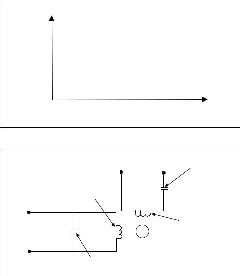
	Fixed Reference	Phase-shift
	Voltage	Capacitor
	Control
	Winding (A)
Control		Reference
Voltage	C	Winding (B)
Va
	Rotor
	Tuning
	Capacitor
Figure 10-16. Two-phase AC induction motor

source of fixed voltage and frequency. This is generally the 60-Hz AC power. The second winding A, the control winding, is powered from the same voltage source of the same frequency, but shifted by 90o in electrical phase. The currents through the two-stator windings produce lines of magnetic flux that pass through the rotor. These magnetic flux lines combine, and at any instant the effect of all the lines can be represented by a single vector that has some annular position relative to the axis of the rotor. As the amount of the currents change at successive instants, the vector angle changes. The result is a magnetic field that rotates at the frequency of the applied voltage. This is indicated in Figure 10-17 at four successive times: t1, t2, t3, and t4. As the lines of flux rotate, they cut across

300 Measurement and Control Basics

the rotor bars, which induce currents in the bars. These electric currents, in turn, produce a magnetic field that reacts with the stator magnetic field and causes the rotor to turn smoothly and continuously.

	Current		Control winding A current
	+					Reference winding B current
										Time
	_
	t1	t2	t3		t4
_			_			0		+
B			B			B		B
+	0	0	+	_	+	_	+	_	_	+
	A				A		A			A
	t				t2		t3			t4
	1

Figure 10-17. Rotation of a magnetic field in a two-phase motor

The method that is used in control system applications is to make the control winding voltage variable. The resultant motor characteristics are shown in the speed-torque curves of Figure 10-18. These curves show that the stall torque is proportional to the control voltage.

The effect of load torque is to reduce the motor’s speed, which causes a greater difference in speed between the rotating magnetic field and the motor. The induced magnetic field will increase with this difference, creating additional torque to pull the load but at a lower speed. Although the internal effects of rotor slowdown are somewhat more complex in the induction motor than in the DC motor, the external effects are about the same.

In the discussion that follows, we will consider the speed-torque characteristics of the AC motor to be linear (see Figure 10-18). Using this assumption, you can derive AC motor constants that are similar to those of the armature-controlled DC motor. This can be demonstrated by the following example.

In two-phase AC induction motors, a tuning capacitor is added in parallel with the control winding (see Figure 10-18) to help match the output

Chapter 10 – Final Control Elements

301

Torque, oz-in.
6	Va = 100v
5	Va = 75v
4
3	Va = 50v
2	Va = 25v
1
	1	2	3	4	5
					Speed, rpm x 103

Figure 10-18. Speed-torque curves of AC motor

impedance of the control circuit to the input of the AC motor. The capacitor is normally chosen to produce a unity power factor, so the parallel resonant circuit will have a very high input impedance (i.e., minimum power drain on the control circuit). The equation for finding the input tuning capacitor that is required to obtain a unity power factor is as follows:

C =	X L	(10-21)
	2π fZ 2

where

C	=	capacitance in farads
XL	= the inductive reactance of the control winding (Ω)
Z	= the impedance of the control winding (Ω)
f	=	the frequency of excitation (Hz)

Example 10-8 illustrates how to calculate the value of parallel capacitance that is required to make a AC inductive motor winding appear to be purely resistive.

The traditional method for obtaining the necessary 90o phase shift between the two motor currents is to use a phase-shifting capacitor in series with the reference winding, as shown in Figure 10-16. The correct value for this capacitor is normally given in the motor’s engineering specifications.

302 Measurement and Control Basics

EXAMPLE 10-7

Problem: Determine the torque (Kt) and damping constants (Dm) for the AC motor whose speed-torque curves are shown in Figure 10-18. Assume linear operation at a control voltage of 25v.

Solution: Since we are assuming linear motor operation, Equation 10-18 for torque constant reduces to the following:

Kt = Ts

Va

Obtaining the stall torque of 2 oz-in. for a control voltage of 25v from Figure 10-16, we determine the torque constant as follows:

Kt = 2oz − in.

25v

Kt = 0.08 oz-in./v

The damping constant is given by Equation 10-20 (Dm = Ts/Snl). Obtaining a speed of 2,500 rpm for a control voltage of 25v from Figure 10-18, we calculate the damping constant as follows:

	Dm =		2.0oz − in.
		(2.5x103	rev	)(	1min	)(	2π	− rad	)
			min 60s					rev

Dm = 7.64x10−3 oz − in./ rad / s

Another factor you should consider in AC and DC motor applications is the static friction associated with the armature. This requires that a minimum control voltage be applied to rotate the armature. Static friction represents a form of dead-time error in the control system, which degrades system performance. It causes system insensitivity since the controller must develop enough output voltage to overcome the static friction. The static can be expressed as a torque and is generally between 1 and 10 percent of the rated torque of the motor.

Pumps

Pumps are used extensively in liquid flow control system applications because they are simple to operate, are energy efficient, and can provide

Chapter 10 – Final Control Elements

303

EXAMPLE 10-8

Problem: A 60-Hz two-phase induction motor has a control field winding impedance of 100 Ω and a control winding inductive reactance of 150 Ω. Find the value of parallel capacitance that is required to make the winding appear purely resistive.

Solution: Use the equation for the input tuning capacitor that produces a unity power factor as follows:

	C =	X L
		2π fZ 2
C =	150		= 40µ farads
	2(3.14)(60)(100)2

both flow and pressure control in a single piece of equipment. The types of pumps most commonly used in process control systems are centrifugal, positive displacement, and reciprocating.

Centrifugal Pumps

The centrifugal pump is the most widely used process fluid-handling device. It is generally operated at a fixed speed to recirculate or transfer process fluids. If your process requires controlled fluid flow, a control valve is generally installed in the discharge line. However, a control valve is an energy-consuming device. In some applications, this energy loss cannot be tolerated, so a variable-speed drive is used to control the pump.

A centrifugal pump imparts velocity to a process fluid. This velocity energy is then transformed mainly into pressure energy as the fluid leaves the pump. The pressure head (H) that is developed is approximately equal to the velocity at the discharge of the pump. We expressed this relationship earlier during our discussion of fluid flow in Chapter 9. It is given by the following:

		H =	V 2	(10-22)
			2g
where
H	=	pressure head (ft)
V	=	velocity (ft/s)
g	=	32.2 ft/s

304 Measurement and Control Basics

We can obtain the approximate head of any centrifugal pump by calculating the peripheral velocity of the impeller and substituting this velocity into Equation 10-22. The formula for peripheral velocity is as follows:

V = π dω

(10-23)

where

d	= diameter (m or in.)

ω= angular speed (rad/s or rpm)

In English units, velocity is normally expressed in feet per second and angular velocity in revolutions per minute, so Equation 10-23 can be converted into English units as follows:

V [ ft / s] =			3.14ω				d
	12in.						60s
	1 ft				1min .
V [ ft / s] =			ω d				(10-24)
	229

where

d	= impeller diameter (in.)

ω= the angular velocity (rpm)

The following example illustrates how to use Equation 10-24 to determine the velocity of fluid from a centrifugal pump.

Positive-Displacement Pumps

Positive-displacement pumps can be divided into two main types: rotary and reciprocating.

Rotary Pumps

Rotary pumps function by continuously producing reduced-pressure cavities on the suction side, which fills with fluid. The fluid is moved to the discharge side of the pump, where it is compressed and then discharged from the pump. In most cases, flow is directly proportional to pump speed. Therefore, the control system only needs to control the pump speed to control the process fluid flow. This type of pump provides accurate, uniform flow and a minimized power requirement.

To help maintain a constant ∆P across the pump, you can hold pressure on the suction side constant by using a small storage tank with a level con-