

Measurement and Control Basics 3rd Edition (complete book)
.pdfChapter 10 – Final Control Elements |
305 |
EXAMPLE 10-9
Problem: Determine the total head developed in feet by a centrifugal pump that has a 12-in. impeller and is rotating at 1,000 rpm.
Solution: Use Equation 10-24 to find the fluid velocity in feet per second:
V = ω d
229
= (1000)(12) =
V 52.4 ft / s 229
Then, use Equation 10-19 to find the total head developed by the pump:
H = V 2
2g
= (52.4 ft / s)2
H
2(32 ft / s2 )
H = 42.9 ft
troller, as shown in Figure 10-19. You can hold this discharge pressure constant by pumping fluid to the top of the delivery tank. A low-slip pump delivers nearly all its internal displacement in each pump revolution and meters fluid accurately.
Three types of rotary pumps are used for flow control: gear pumps, circumferential piston pumps, and progressing cavity pumps. Gear pumps are used to pump high-viscosity fluids or to generate moderately high differential pressures. Because these pumps have close gear-to-gear contact, they are used for clean, nonabrasive lubricating fluids.
Circumferential piston pumps are widely used in sanitary and food applications. This type of pump has two noncontacting fluid rotors. Because the sealing area is relatively long, slip is nearly eliminated at viscosities above 200 centistokes. Flow control applications include pumping dairy and bakery products, plastics and resins, and pharmaceuticals. These pumps cannot be used to pump large solids or extremely abrasive fluids or in high-back-pressure applications.

306 Measurement and Control Basics
LC |
LT |
100 |
100 |
LV |
|
100 |
|
Small storage |
|
Tank |
|
LE |
Process |
100 |
|
Fixed |
Tank |
|
|
Level |
|
|
PD Pump |
Figure 10-19. Positive displacement (PD) pump application
In the progressing cavity pump, a single helical rotor turns eccentrically in a stationary stator. As the rotor turns, cavities are produced, which are filled at the inlet by the process fluid and move through the stator to the discharge side of the pump.
Reciprocating Pumps
Reciprocating pumps use a linear reciprocal stroke in combination with check valves to pump fluid. Reciprocating pumps are commonly used to control the rate at which a volume of fluid is injected into a process stream or vessel. These pumps are also called metering pumps in some applications because they are highly accurate and consistent in the volume of fluid discharge per cycle. Large reciprocating pumps generally have vari- able-speed drives. Small, controlled-volume reciprocating pumps used for precise chemical injection normally use a variable-stroke controller.
The two basic types of reciprocating pumps normally used in metering applications are plunger pumps and diaphragm pumps. In the plunger pump, a packed plunger draws in and then expels fluid through a oneway check valve. A diaphragm-reciprocating pump can be mechanically driven, directly coupled to a plunger, or hydraulically actuated. Like the
Chapter 10 – Final Control Elements |
307 |
plunger pump, it draws in a precise amount of fluid and discharges it cyclically.
EXERCISES
10.1An equal percentage valve has a maximum flow of 80 gal/min and a minimum flow of 5 gal/min. Find its rangeability.
10.2Assume that a force of 200 N is required to fully open a control valve equipped with a diaphragm valve actuator. The valve input control signal connected to the actuator has a range of 3 to 15 psi. Find the diaphragm area that is required to fully open the control valve.
10.3Describe the procedure valve manufacturers use to determine the valve-sizing coefficients (Cv) for their valves.
10.4A liquid with a specific gravity of 0.9 is pumped through a pipe that has an inside diameter of 18 in. at a velocity of 10 ft/s. Find the volume flow rate.
10.5Calculate the Cv, and select the required valve size from Table 10-1 for a valve with the following service conditions:
Fluid: ethyl alcohol (SG = 0.8)
Flow rate: 200 gal/min
P1: 100 psi
P2: 90 psi
10.6An 8-in. control valve is operated under the following conditions:
Fluid: water
Flow rate: 800 gal/min Temperature: 70°F
Pv: 0.36
P1: 100 psia
P2: 90 psia rc: 0.95 Km: 0.6
Determine whether the valve will cavitate under these service conditions, and then calculate Cv.
10.7Describe the basic difference between flashing and cavitation in control valves.
308Measurement and Control Basics
10.8Determine the torque and damping constants for the armaturecontrolled DC motor whose speed-torque curves are shown in Figure 10-14. The armature voltage is 28 v.
10.9Determine the torque (Kt) and damping constants (Dm) for the AC motor whose speed-torque curves are shown in Figure 10-18. Assume linear operation at a control voltage of 50v.
10.10A 60-Hz two-phase induction motor has a control field winding impedance of 200 Ω and a control winding inductive reactance of 250 Ω. Find the value of parallel capacitance that is necessary to make the winding appear purely resistive.
10.11Calculate the total head in feet that is developed by a centrifugal pump with a 10-in. impeller and that is rotating at 800 rpm.
10.12Explain the basic operation of a positive-displacement rotary pump.
BIBLIOGRAPHY
1.Driskell, L. Control-Valve Selection and Sizing, Research Triangle Park, NC: ISA, 1983.
2.Fischer, K. A., and D. J. Leigh. “Using Pumps for Flow Control,” Instrument & Control Systems Magazine, March 1983.
3.Control Valve Handbook, 2d ed., Fisher Controls Company, 1977.
4.Johnson, C. D. Process Control Instrumentation Technology, 2d ed., New York: John Wiley & Sons, 1982.
5.Murrill, P. W. Fundamentals of Process Control Theory, 3rd Ed., Research Triangle Park, NC: ISA, 2000.
6.Weyrick, R. C. Fundamentals of Automatic Control, New York: McGrawHill, 1975.


310 Measurement and Control Basics
decided to market its computer as a process control computer, repackaging it as the RW-300. This was a very important entry in the early history of process computers. It is interesting to note that computer control developed not as an initiative of the process and manufacturing industries but as a result of computer and electronics vendors efforts to expand their markets beyond military applications.
The first industrial installation of a computer system was made by the Daystrom Company at the Louisiana Power and Light plant in Sterlington, Louisiana. It was not a closed-loop control system, but rather a supervisory data-monitoring system (see Figure 11-1).
Data and Alarm
Output Devices
Digital
Computer
Process
Figure 11-1. Supervisor data-monitoring system
The first industrial closed-loop computer system was introduced in March 1959 at the Texaco Company’s Port Arthur, Texas, refinery using an RW-300. The first chemical plant control computer was unveiled at the Monsanto Chemical Company’s ammonia plant in Juling, Louisiana, in April 1960. It also used an RW-300 to achieve closed-loop control.
The next major advance in process control computers came with the introduction of programmable logic controllers (PLC). In 1968, a major automobile manufacturer wrote a design specification for the first programmable logic controller. The primary goal was to eliminate the high cost of frequently replacing inflexible relay-based control systems. The automaker’s specification also called for a solid-state industrial computer that could be easily programmed by maintenance technicians and plant engineers. It was hoped that the programmable controller would reduce production downtime and provide expandability for future production changes. In response to this design specification, several manufacturers developed logic control devices called programmable controllers.
Chapter 11 – Process Control Computers |
311 |
The first programmable controller was installed in 1969, and it proved to be a vast improvement over relay-based panels. Because such controllers were easy to install and program, they used less plant floor space, and they were more reliable than relay-based systems. The first programmable controller did more than meet the automobile manufacturer’s production needs. Design improvements in later models also led to the wide-spread use of programmable controllers in other industries.
Two main factors in the early design of programmable controllers appear to have caused their success. First, designers used highly reliable solidstate components, and the electronic circuits and modules were designed for the harsh industrial environment. The system modules were built to withstand electrical noise, moisture, oil, and the high temperatures encountered in industry. The second important factor was that the programming language designers initially selected was based on standard electrical ladder logic. Earlier computer systems failed because it was not easy to train plant technicians and engineers in computer programming. However, most were trained in relay ladder design, so they could quickly learn to program in a language based on relay circuit design.
When microprocessors were added to PLCs in 1974 and 1975, they greatly expanded and improved the basic capabilities of programmable controllers. They were now able to perform sophisticated math and data-manipu- lation functions.
In the late 1970s, improved communications components and circuits made it possible to place programmable controllers thousands of feet from the equipment they controlled. As a result, most programmable controllers could now exchange data, meaning they could more effectively control processes and machines. Also, microprocessor-based input and output modules enabled programmable controller systems to evolve into the analog control world.
Programmable controllers can be found in thousands of industrial applications. They are used to control chemical processes and facilities. They are also found in material-transfer systems that transport both raw materials and finished products. PLCs are now used with robots to perform hazardous industrial operations, making it possible for humans to perform more intellectually demanding functions. Programmable controllers are used in conjunction with other computers to collect and report process and machine data, including such uses as statistical process control, quality assurance, and diagnostics. Finally, they are also used in energy-manage- ment systems to reduce costs and improve the environmental control of industrial facilities and office buildings.
Chapter 11 – Process Control Computers |
313 |
Direct digital control was achieved by Imperial Chemicals Industries, Ltd., in England, using an ARGUS 100TM computer built by the Ferranti Company and installed in a soda ash plant in Fleetwood, Lancastershire. At the same time but independently, the Monsanto Company achieved DDC with an RW-300 computer in its ethylene plant at Texas City, Texas. The Monsanto installation was under closed-loop control in March 1962, where it controlled two distillation columns. The Imperial Chemicals system was installed in the summer of the same year.
The success of these early DDC installations generated a great deal of interest in the user and vendor communities alike. As a result, the Instrument Society of America established the DDC Users Workshop in 1963. The ISA’s Guidelines and General Information on User Requirements Concerning Direct Digital Control is generally credited with having played a major role in the development of the minicomputer for process control.
The DDC system has always had the potential to be used for an unlimited variety and complexity of the automatic control functions in each and every control loop. However, the vast majority of DDC systems were implemented as digital approximations of the conventional three-mode analog computer.
The Centralized Computer Concept
The early digital computers had many disadvantages. The most significant was their slowness. For example, performing math addition commonly took 4 ms. Another disadvantage was that computer memories were very small; typically, they were able to store only four to eight thousand words of only eight to sixteen bits each. Limited software capability was another problem. All programming had to be done in machine language since assembly language or higher-level languages had not yet been designed or written in the early stages of process computers. A fourth problem was that neither instrument vendors nor user personnel had any experience in computer applications. Thus, it was very difficult to properly size projects within a computer’s capabilities; most had to be reduced to fit the available machines. Another very significant disadvantage was that most of the early computer systems were very unreliable, particularly if they used germanium rather than silicon transistors. To operate effectively, computers in this period depended on unreliable mechanical devices (air conditioners).
The response of computer manufacturers to these deficiencies was to design a much larger computer system in which arithmetic functions were designed in the magnetic core memory. These changes made the computers much faster, but, because of the high cost of core memories and the

314 Measurement and Control Basics
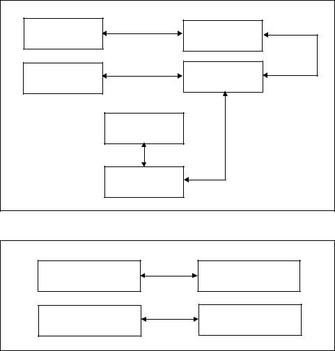
additional electronic circuitry, they also were much more expensive. In addition, to help justify this cost the vendors promoted the incorporation of all types of computer functions, including both supervisory control and DDC, in one computer mainframe at a central control room location (Figure 11-4).
|
Centralized Computer System |
|
Supervisor’s Console |
Supervisory |
|
Control Computer |
||
|
||
Operator’s Console |
Direct Digital Control |
|
DDC Computer |
||
|
||
|
Process |
Figure 11-4. Supervisory plus direct digital control
Although these computers greatly alleviated the speed and memory problems of the earlier systems, they led to other problems. Most computer systems were sold and installed before their designs were thoroughly proved or their programming aids (compilers, higher-level languages, etc.) fully developed. Thus, the users who tried to install them experienced many frustrating delays. Because of the centralized location of these computers, it was very expensive to install the vast plant communication system required to bring the plant signals to the computer and return control signals to the field. Moreover, unless this plant communication system was carefully designed and installed, it was prone to electrical noise problems.
Because all the control functions were located in one computer, users feared the ramifications of that computer’s failure and demanded a complete analog backup system that paralleled the DDC. The system that resulted is shown in Figure 11-5. To compensate for these high costs, users and vendors alike tried to squeeze the largest possible projects into the computer system, drastically complicating its programming and installation.
Because of these problems and failures many companies’ management reacted quite negatively to computer control and the installation of computer systems slowed until about the mid-1970s.