О.И. Никонов

М.А. Медведева

Electronic text edition

ABSTRACT OF LECTURES

on the module "Mathematics for economists (the advanced level, partially in English): "Mathematical modeling" for the masters who are trained in the directions

080100 Economy

080200 Management

080500 Business informatics

230700 Applied information scientists

1230400 Information systems and technologies

010300 Fundamental information scientists and information technologies

Yekaterinburg 2011

СОДЕРЖАНИЕ

LECTURE 1-4. IMITATING MODELLING 4

Introduction 4

Consent criteria χ2 8

By (14) we can estimate the required number of passes N to achieve the desired accuracy. 18

Определение цены опциона методом имитационного моделирования 20

Общие принципы имитационного моделирования многокомпонентных систем 22

Организация квазипараллелизма просмотром активностей 23

Два способа изменения (протяжки) системного времени 26

Организация квазипараллелизма транзактным способом 31

Испытание и эксплуатация имитационных моделей 33

Верификация и проверка адекватности модели 34

Верификация 34

Проверка адекватности модели 34

Оценка погрешности результирующего показателя имитации из-за различия затравочных чисел генератора псевдослучайных чисел 35

Методы понижения дисперсии 36

Антитетический метод 36

Понижение дисперсии при вычислении интегралов 37

Применение имитационного моделирования (ИМ) к сравнению методов оценивания и анализу их точности 38

Основная литература 41

Дополнительная литература 41

Лекция 5-9. Эконометрическое моделирование 43

Обобщенная линейная модель множественной регрессии 43

Обобщенный МНК 45

Прогноз в ОЛММР 49

Дихотомические результирующие показатели. Логит- и пробит-модели 49

Маржинальный эффект фактора 52

Стохастические объясняющие переменные 52

Адекватность моделирования. Состоятельные методы 55

Оптимальный предиктор 56

Алгоритм чередующихся математических ожиданий – ACE-алгоритм (alternating conditional expectations) 58

Проверка адекватности моделирования 61

Скользящий экзамен (cross-validation) 63

Процедура bootstrap 63

Модели с лаговыми переменными 63

Полиномиальная лаговая структура Алмон 65

Геометрическая лаговая структура Койка 67

Модель частичной корректировки 68

Модель адаптивных ожиданий 70

Модель потребления Фридмена 71

Основная литература: 72

Дополнительная литература: 73

LECTURE 1-4. IMITATING MODELLING

Introduction

Receipt of the decision on mathematical model can be:

• deductive, i.e. from general mathematical properties, theorems, laws the solution of a private task is found (the decision in an analytical type);

• imitating (the accelerated playing of process on the computer).

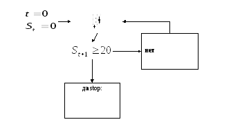
Example 1.1. The person passed 20 km with a speed of 4 km/h. What time it spent?

According to the law of uniform motion (mathematical model).

We will receive the deductive decision, having divided both parts into v:

.

Imitation: we will designate the way passed by the time of t time for St. In each hour the way increases by 4 km. We will look, by what moment 20 km will be gained. We constitute algorithm (flowchart), we code it in any programming language, we start the program and we find the same answer: t * = 5 h.

In case of difficult system to construct the model allowing the deductive decision happens difficult or it is impossible. Then resort to imitating modeling.

Definition. Imitating modeling – a series of the numerical experiments urged to receive empirical estimates of extent of influence of factors on the results depending on them. Imitating modeling using random numbers is called a Monte Carlo method (the city in Monaco – the principality between France and Italy, – famous for gaming houses).

According to one Internet overview, in case of the problem resolution of management of firms the following methods are most often used:

1. imitating modeling (29%);

2. linear programming (21%)

3. network planning methods and managements (14%);

4. management theory inventories (12%);

5. nonlinear programming (8%);

6. dynamic programming (4%);

7. integer programming (3%);

8. theory of queues (systems of mass servicing) (3%);

9. other (6%).

Probabilistic and statistical aspects of imitating modeling

Often mathematical models of the systems interesting us contain accidental parameters of their functioning and/or accidental external impacts.

Example 2.1. Work of a hairdressing salon is researched. Accidental external impacts – time intervals between the next visitors δ1, δ2, …. Accidental parameters of functioning – times τ1 (l), τ2 (l), … servicing of the next clients of l – m the hairdresser. A research purpose – to solve, how many to hire hairdressers that the average time of expectation in queue didn't exceed the set size. For this purpose it is necessary to lose some working days (are accelerated) and to look what will be queue in case of different number of hairdressers. To lose day of work, it will be required to generate specific values d1, d2, … sizes δ1, δ2, …. We will consider that δ1, δ2, … – the independent, equally distributed random variables: i.e. d1, d2, … – implementation of selection of distribution.

For some random variables, we will tell δ, we assume a certain type of distribution, for example exponential, for others (τ1 (l)) a type of distribution isn't clear, and there is a task of check of a hypothesis that this some fixed (standard) distribution which we assume.

Criterion of a consent of Kolmogorov

The main ("zero") hypothesis consists that function of distribution of a random variable ξ is some fixed function

, (1)

alternative hypothesis – distribution function another:

. (2)

For check of these hypotheses we use selection of supervision of size ξ:

. (3)

Empirical function of distribution:

.

If H₀ is fair, must be close to and backwards, that is size will be indicative – the maximum deviation of empirical function of distribution from the hypothetical. it is accidental, as selection on which is calculated , I could be different. Great values in advantage H₁, therefore significance value of specific data , which led to the specific , against a hypothesis H₀, equals

.

Kolmogorovs Theorem. If is continuous, that distribution of statistics , on condition of justice of Н₀, doesn't depend from also is called as Kolmogorov's distribution with N degrees of freedom.

Example 2.2. On selection to check a hypothesis Н₀: – _{uniform distribution on a piece [1, 5] (U(1, 5)).}

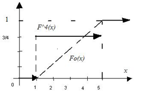
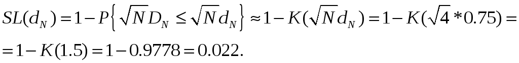
_{From picture}

_{We can see, that d4 = ¾. .}

_{According to tables [7, table 6.2] we find SL <0.01 (0.01 precisely for 0.734). Such significance value of data is interpreted as "the high importance, H0 almost for certain doesn't prove to be true", ξ has no distribution of U(1, 5).}

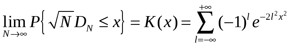
Kolmogorovs Theorem.. .

K(x) is called Kolmogorovs distribution [7, table 6.1] .

already in case of N > 20.

Example 2.2 (continuation):

As empirical function of distribution is step, and not decreasing, then it is the share of one of function gap points .

Consent criteria χ2

_{Hypotheses (1), (2) according to data (3) are again checked. Algorithm of actions:}

_{We will break area of possible values of a random variable ξ on H0 on}

_{r of intervals} k = 1,…, r.

To these intervals on distribution of H₀ there correspond probabilities of hit ξ in them _.

ν_k – number of supervision (sample units) which got to k-y an interval

(), (4)

– frequency of hits in an interval.

Compare statistics . In case of accomplishment of H₀ of frequency will be close to the corresponding probabilities therefore small values of statistics of H² therefore great values witness against H₀ are expected.

, – the observed (actually received) value of statistics of H².

Pearsons Theorem.

In case of justice of H0 distribution of statistics of H2 aims in case of to distribution χ² with r – 1 degrees of freedom.

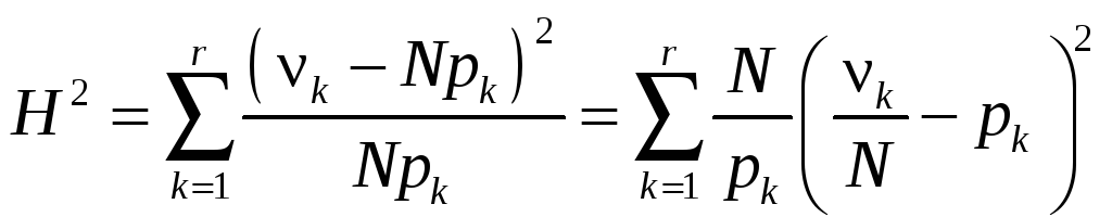
Heuristic proof:

according to Moivre – Laplace theorem

,

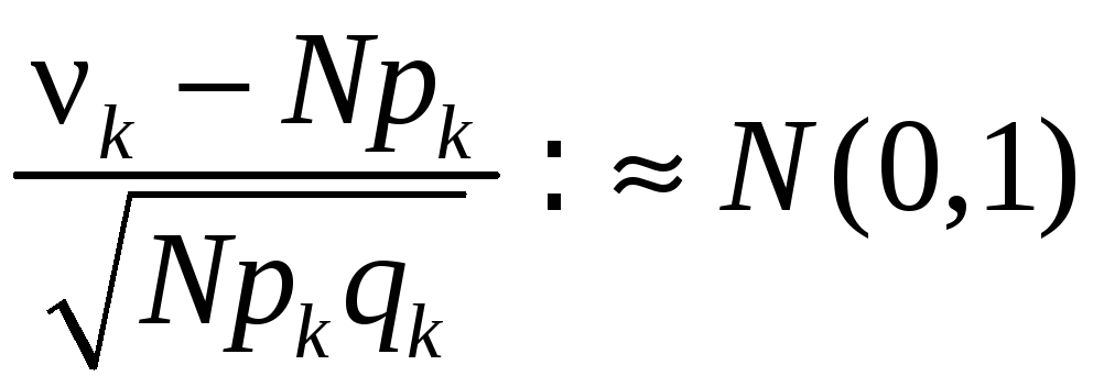, that is has distribution χ2 with r freedom degrees (actually r – 1 as on (4) νr depends on the others).

According to Pearsons theorem

. (5)

Owing to approximate nature of a formula (5) it is desirable to provide , , n_k – numbers of sample units in intervals (can be, for this purpose it is necessary to unite intervals).

If it isn't completely determined and l of its unknown parameters were estimated on initial selection, the number of degrees of freedom in (5) needs to be reduced to r – 1 – l.

Definition. Diagram like function from – average points of intervals, is called as the histogram.

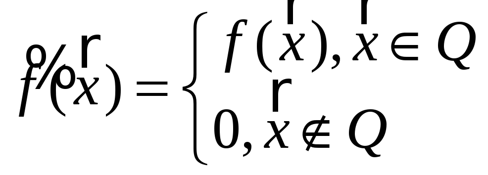
We will check H₀ hypothesis that – normal distribution with the parameters estimated on the same selection (curve fo(y)).

p₁ = F₀(4) – F₀(-∞) = 0.262, p₂ = F₀(5) – F₀(4) = 0.252, p₃ = 0.246, p₄ = 0.156,

p₅ = 0.084.

,

.

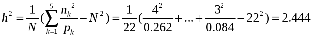SL is great (> 0.1), data aren't significant against H₀, it could be supervision of a normal random variable.

Generation of the pseudorandom numbers which are regularly distributed on a piece [0, 1]

Carrying out imitation will require implementation

(6)

distributions . Distributions will be necessary different, for a start let it will be U(0, 1).

Practically we receive numbers (6) by consecutive appeals to some sensor which can be the physical device connected with a case or the computer program which develops various numbers. In the latter case these numbers call pseudorandom with distribution , if they meet conditions which are expected from selection of distribution . Pseudorandom (allegedly accidental) as truly accidental they aren't (can be always repeatedly received).

Thus, we expect (and it is necessary to check it) from pseudorandom numbers with distribution of U(0, 1):

– uniformity, i.e. consent with distribution of U(0, 1).

– accident.

Criterion of accident

Let there is an ordered set of numbers

(7)

(or a train – final sequence).

Definition. The train is called accidental if it is selection implementation.

According to data (7) it is necessary to check a hypothesis ,

that is the independent equally distributed random variables, in case of alternative of H₁ it not so.

We will consider in the beginning a case when elements in (7) can be only two types (1 and 0, And and In,…).

Example 2.7. Train 10100011010.

In really random check of this kind we don't expect that all "1" will get off together, and we don't expect that they will regularly alternate with "0".

In a train of elements of two types the set of the going in a row identical elements limited to opposite elements, either the beginning, or end is called as a series.

As statistics of criterion we will choose a random number of series K. We will designate: N₁ – number of elements than which in a train it is less; N₂ – number of elements than which in a train it is more.

It is possible to show that in case of justice of H₀ . Means, strong deviations of number of series from MK – for benefit of H₁ hypothesis.

SL(k) = P { K = k or further away from MK (all "tail") + K belongs to opposite "tail" with the same probability | H₀ }.

In case of the fixed SL = α it is possible to tabulate sizes и such that in case of the reached SL will be > α.

Example 2.7 (continuation): N₁ = 5, N₂ = 6, number of series k = 8.

According to the table of distribution of K [7, table 6.7]:

=> SL > 0.05;

=> SL > 0.1.

Means, SL> 0.1, data aren't significant against H₀, the train is accidental.

If either N₁, or N₂> 20, statistics

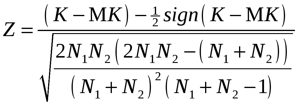in case of H₀ has normal standard distribution is approximate. Therefore

. (8)

Now let numbers (7) – allegedly selection of arbitrary continuous distribution. It is possible to resolve an issue of not accident of this train as follows.

We will remember: a median – a quantile about 0.5; the selective median of Me is equal to a median element of a variational series if number of supervision odd, and it is equal to a floor the amount of 2 median elements of a variational series if number of supervision even. We will constitute differences 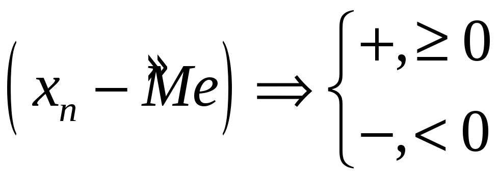, then instead of (7) we have a train of signs + and – which accident we are able to check.

If the train (7) accidental, consecutive excess of a median is independent events and the train of signs will be accidental therefore if a train of signs the nonrandom, and initial train wasn't accidental.

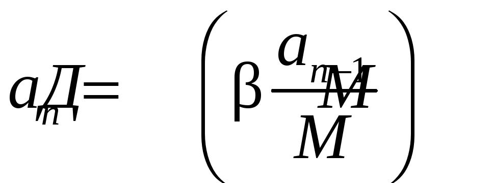
Multiplicative congruent method generation pseudorandom Numbers

Let x _n -1 - a number (0, 1). Obtain , Where β - large integer; D - taking the fractional part (discard the integer part, if there is one). The new number x _n Again from (0.1) it again multiplied by β and t. d., get the sequence of numbers uniformly distributed nnyh g on (0, 1).

The algorithm can be rewritten. Let a _n - integer, M - large integer,

, (9)

. (10)

Definition. Alance of the division of a natural number p by a positive integer q denotes (p) mod q.

Formula (10) can be rewritten

, n = 1, 2, …. (11)

 algorithm is (11), (9) easier to implement on a computer.

The sequence P (11) always loops, ie. e. beginning with some n = ₀ to the period length T, which then repeats endlessly smiling. L - length of the segment aperiodicity.

Simulation of a discrete random variable

Need to get the implementation of sample of η:

y^(^r^)			…
			…

- distribution law.

 

Depict the probability of this law on the real axis.

Next comes the uniform "shooting" over the interval [0, 1]:

1) n = One;

2) is generated by x _n - Implements a tion

;

3) announced the implementation of the value η ;

Since ξ    uniformly distributed on [0, 1], the values ​​I   y ^(r) will appear with a probability equal to the length of the segment  ,_., Vol. e. p _r

Simulation of a continuous random variable with an arbitrary distribution

Suppose we have to get the implementation of sample of η:  is a given with m cerned monotonically increasing function.

Theorem (The inverse function). Let inverse function. If ξ ~ U (0, 1), , Then the random variable η will have a (right) distribution _.

Proof: =

=.  The third equality holds, as the case of strictly monotonically increasing transformation sign of inequality persists. The last equality is obvious from the figure.

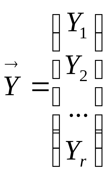
Simulation of random vectors

Suppose you want to generate a sample N values ​​of the random vector with predetermined characteristics:

expectation and covariance matrix .

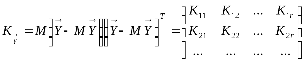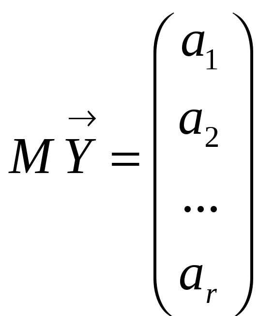
Express the vector 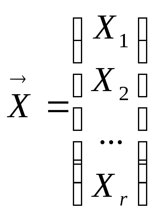  with independent, identically distributed components   with independent, identically distributed components

 For example, for r = 2, we write:

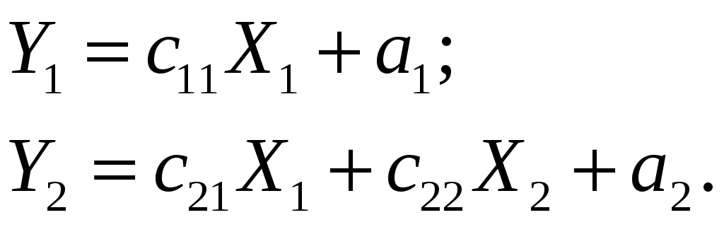(12)

viously, Y ₁ and Y ₂ have the desired mat ematicheskie expectations. I f = 0, then they are functionally (fully) dependent, if = 0 , then they are not dependent

We choose o that Y ₁ and Y ₂ and had the desired standard deviation and correlation coefficient.

Statistical analysis of simulation results

Once we have taken care of properly distributed randomness and random external influences and / or parameters of the model, our model bude t "live" almost real life and fix a variety of e f values ​​from run to run - it's like watching a real system repeatedly. This means that these data can be recorded and shall apply the whole arsenal of mathematical statistics to estimate the nature ISTIC quantities of interest, their dependence on it (correlation), and so on. D.

Examples of simulation

A simple system with the influence of the external environment

Example 4. One. It is known that the system is affected by the input random variable L ~ U (- 1, 2) and affects the external environment, the random variable F ~ N (2, 1). We are interested in the output value

.

What about Y? Clearly, this is a random variable whose distribution is deductively very difficult to find. First of all, we are interested in the expectation MY. To estimate the expectation generate a sample What about Y? Clearly, this is a random variable whose distribution is deductively very difficult to find. First of all, we are interested in the expectation MY. To estimate the expectation generate a sample 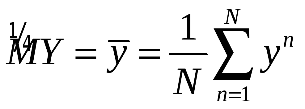.  Algorithm: Generate sample ; Generation sample ; For n = 1 , ..., N, .

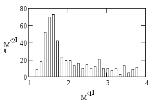If we make a simulation with N = 500, we obtain the estimate the expectation ,  Estimate the standard deviation .  Histogram gives an idea of the distribution of the output variable Y. In particular fashion near 1.5 and m. G.

The confidence estimate of the error of simulation calculations

If the goal is to find the expectation MY, you can specify the error of its determination. According to the central limit theorem, for large N, regardless of the distribution of Y:

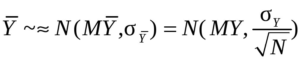• . Hence,  can not occur further away

• from the MY, than standard deviations:  , Equivalent

. (14)

Here, the factor 2 corresponds to a confidence level of 0.954, and 3 - 0.997.

Example 4. 1 (continued). Replacing the standard deviation of its estimate , We obtain:  with a probability of 0.954.

By (14) we can estimate the required number of passes N to achieve the desired accuracy.

Calculation of certain multiple integrals and Monte Carlo

Suppose you want to calculate the integral defining g nny. Recall the mean value theorem. .  Point c is unknown. What if we take e f randomly, uniformly distributed on the interval g constant of integration?

с → ξ ~ U(a,b).  then the result value and the mean value theorem will be random: η = (b - a) f (ξ). What is his expectation?

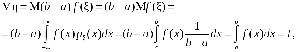
ie coincides with the desired integral!

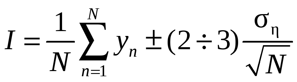
We know that the expectation of a random variable can be estimated with an accuracy controlled by it generated sample (14), so

, ~ U(a, b); (15)

, (16)

:can be roughly estimated from the top: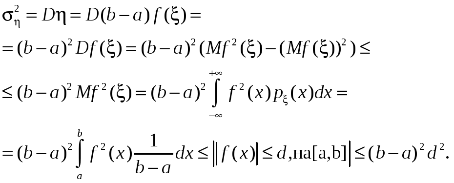

. ₍₁₇₎

Or replaced by the estimate of the standard deviation of the sample (15).

Example 4. 2 Calculate the integral.

_{Use the number t n, a uniformly distributed on [0, 1] from the table of random numbers. Of these, we obtain x n ~ U (0, π / 2).}

n	1	2	3	4	5	6	7	8	9	10
tn	0.1	0.09	0.73	0.25	0.33	0.76	0.52	0.01	0.35	0.86
xn	0.157	0.141	1.147	0.393	0.518	1.194	0.817	0.016	0.55	1.351
yn	0.621	0.59	1.5	0.972	1.106	1.515	1.341	0.197	1.135	1.552

According to the formula (16) with a confidence level of 0.954. By (17) <= 1.57. In this example, we can give a more accurate estimate:  <= 1.253. So I = 1.05 ± 0.79.

A summary of the sample = 0.46, then I = 1.05 ± 0.29.

Sometimes the error of taking the probable error, 0.674 instead.  Its meaning is that the probability that the actual error is greater in absolute value of the error or less identical (= 0.5). Then I = 1.053 ± 0.098

Если нужно вычислить кратный интеграл , где V – s – мерный куб, то расчет идёт по формуле (16), где , выборка из – равномерно распределённого в кубе V случайного вектора; оценивается аналогично.

Для вычисления , где Q:

введём , тогда .

Метод Монте-Карло экономнее в вычислениях, чем квадратурные формулы в случае кратных интегралов, и проще учитывает сложную форму области интегрирования Q.

Определение цены опциона методом имитационного моделирования

Опцион на покупку – документ, дающий право, но не обязательство на покупку актива по указанной в нём цене (цена исполнения) в указанную в нём дату (момент исполнения).

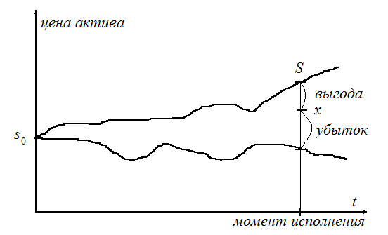
Если пренебречь инфляцией, т. е. не рассматривать дисконтирование, то ясно: выгода от обладания опционом на момент исполнения (ценность опциона) – это цена актива на момент исполнения S минус цена исполнения x. Поскольку владелец опциона может отказаться от него без последующих обязательств, ценность опциона не может быть отрицательной:

V = max(S – x, 0).

Цена актива S случайна, значит, и ценность V случайна, и ценой опциона, т. е. тем, что за опцион стоит отдать в момент покупки, надо считать по определению MV – математическое ожидание ценности.

Как образуется S ? Будем считать, что цена актива непрерывно наращивается с однодневной ставкой R₁. Значит, через один день цена актива . Для одногодичного опциона (250 торговых дней) . Для простоты считаем R_t независимыми, одинаково распределёнными величинами.

Для определения MV с заданной точностью применим имитационное моделирование: нужно получить N «наблюдённых путем проигрывания» модели значений vⁿ , и . Здесь vⁿ = max(sⁿ – x, 0), и для получения конечной цены актива в n-м прогоне генерируется 250 значений однодневных ставок rⁿ_t. При этом используется эмпирическое распределение, построенное по многодневным наблюдениям за однодневной ставкой.

Общие принципы имитационного моделирования многокомпонентных систем

Система – совокупность объектов, объединённых некоторой формой регулярного взаимодействия или взаимозависимости для выполнения заданной функции. Отдельные элементы системы или её подсистемы называются компонентами.

Пример 1. Движение эскадрильи самолётов на учениях. Каждый i-й самолёт – компонента системы, в его движении можно выделить ряд стадий, в ходе которых выполняется последовательность функциональных действий (ФД). При t_i0 начинается взлёт i-го самолёта со взлётной полосы – это функциональное действие ФД_i1. Разгон и боевой разворот – ФД_i2. Стрельба по мишени – ФД_i3 и т. д.

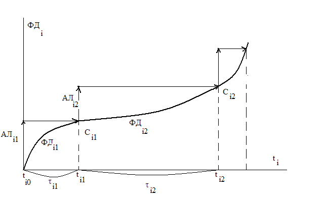
Любое ФД_ij выполняется на интервале τ_ij и завершается событием С_ij. Для каждой i-й компоненты вводится своё локальное время t_i.

В имитационной модели ФД_ij аппроксимируется некоторым упрощённым функциональным действием (алгоритм АЛ_ij), который реализуется при неизменном значении t_i , а затем осуществляется изменение t_i на τ_ij, инициируя появление события С_ij. Пара (АЛ_ij, τ_ij) = АК_ij – активность (работа).

Если бы на компьютере имитировалось поведение только одной компоненты, то выполнение активностей можно было бы осуществлять строго последовательно, пересчитывая каждый раз t_i. На самом деле компонент много и функционируют они одновременно, а в большинстве компьютеров в каждый конкретный момент может исполняться алгоритм только одной из компонент модели. Необходимо реализовать квазипараллелизм – выстраивание параллельно происходящих активностей в последовательный порядок, с учётом их должной синхронизации (для учёта взаимовлияния). Это делается с помощью глобальной переменной ts – системного времени. Системное время – это мыслимое (в часах, днях, годах) модельное время, в котором происходит эволюция модели. Фактически это последовательность моментов, в которых нужно выполнять какие-либо активности компонент.