

Economic
Operation of Power Systems
Figure
4-1Typical input-output curve of a thermal-electric unit. Input can be
expressed in Btu, equivalent barrels of oil, or Mcf of gas. (An
equivalent barrel is 6,250,000 Btu, and an Mcf of gas may vary
depending on the source but is usually approximately 1,000,000
Btu.)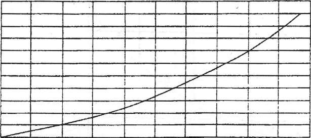
0 10 20 30 40 50 60 70 80 90 100 Output - Magwitts
x
ь
I m1000
о
с
I
400
Figure
4-2Input-output curves for two typical thermal units, though the
no-load fuel for unitВis greater than
that of unit A, at loads above 40 MW the heat input for unit
Вis less than that for unit
A.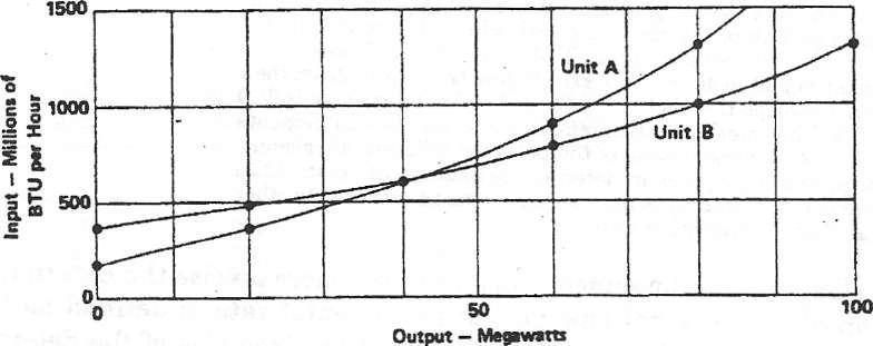
solve this problem have been developed and are in general application throughout the industry.
Consider two 100-MW thermal units Aand Вwith input-output curves as shown in Fig. 4-2.
Incremental Rates
It can be shown mathematically that minimum fuel input for any given total load of the two machines will occur when they are operated at equal incremental heat rates. Because fuel has a cost, such as cents per Btu, dollars per equivalent barrel, or cents per Mcf, the above statement can be modified to say that the minimum cost will occur when the incremental costs are equal.
The term "incremental" merely means a small increase. Of course,
О 10 20 30 40 SO X
Figure 4-3Curve showing determination of incremental changes. For a small distance along a curve it can be considered to be a straight line. The increments on the x axis in this case are from 10 to 20 between points 2 and 3 and from 30 to 40 between points 4 and 5. When following the curve from 10 to 20 on the xaxis, it goes from 6 to 8 on the уaxis. The slope of this portion of the curve is a ratio of the differences or (8 - 6) - (20 - 10), which equals 2/10 = 0.2. When following the curve from 30 to 40 on the x axis, it goes from 14 to 22 on they axis. The slope then is (22 - 14) + (40 - 30), which equals 8/10 = 0.8. This method, using smaller and smaller increments until they approach zero, is the basis for differential calculus. For practical purposes in determining incremental costs, little error is introduced by using reasonably small increments other than those approaching zero.
the smaller the increment (increase), the more precise the determination of incremental change. An incremental rate is defined as the slope of a curve from one point to another. Examples of the determination of incremental rates are given in Fig. 4-3.
An inspection of Fig. 4-3 gives a clue to an easy method of determining incremental rates. If it is assumed that the curve is made up of straight-line segments between the numbered points, then we have already calculated the incremental rates (slopes) for points Вand D. The slope at A would be (6 - 4) + (10 - 0) or 2/10 = 0.2. At pointСthe slope would be (13 - 8) + (30 - 20) or 5/10 = 0.5.
At point E the slope would be (36 - 22) - (50 - 40) = 14/10 = 1.4. An incremental-rate curve is developed by plotting the points determined by the above calculations. This is shown in Fig. 4-4.
Economic Loading of Generating Units
When the basis for determining incremental-rate curves has been developed, this method can be used to determine how to operate electric generating units for minimum production cost. A procedure for determining load allocation for minimum fuel cost between the two
/
И
/
/
У
1 0 О 10 20 30 40 SO
X
2.0
>■ i
о
&1.5
я
£ О
о
• 1.0 т
СС д
|
0.5