The Physics of Coronory Blood Flow - M. Zamir

290 8 Elements of Unlumped-Model Analysis

normalized pressure

2.5
2
1.5
1
0.5
0
-0.5
-1
-1.5
-2
-2.5 0	0.2	0.4	0.6	0.8	1
		normalized distance

Fig. 8.7.1. Wave propagation in a tube can be thought of graphically as a simple sine or cosine wave moving along the tube as time goes on.

Thus, because |eiωt| = 1.0, the amplitude of the travelling wave is always equal to the amplitude of the pressure oscillations in space within the tube, namely |p(x)|, which is a function of x representing the distribution of peak pressure along the tube and we shall refer to it simply as the “pressure distribution” within the tube. It is a key element in the analysis of wave reflections within a tube because it provides a measure of the amount by which the pressure distribution along the tube is modified by wave reflections and hence a measure of the amount by which the flow is being a ected by the moving wave. The reason for this is that in the absence of wave reflections we have, from Eq. 8.7.7 above,

|p(x)| =	cos	ωx	− i sin	ωx		(8.7.13)
		c		c
= 1.0						(8.7.14)

This means that in the present case the pressure peaks reached at di erent points along the tube are equal, as shown graphically in Fig. 8.7.2. That is, the pressure distribution is uniform at a normalized value of 1.0. We shall find this result for the pressure distribution is a singular result in the sense that it can only occur in the absence of wave reflections. Because of this, any deviations from |p(x)| = 1.0 in other cases can be attributed immediately to the e ects of wave reflections.

To see the way in which the pressure distribution along a tube is actually modified by wave reflections, consider a tube of length l in which the following

normalized pressure

8.7 Wave Reflections

291

1.5

1

0.5

0

−0.5

−1

−1.50	0.2	0.4	0.6	0.8	1
		normalized distance

Fig. 8.7.2. The peaks of pressure oscillations at di erent positions along the tube, represented by the bold line, shall be referred to as the “pressure distribution” along the tube. Only in the absence of wave reflections is this distribution uniform at a normalized value of 1.0 as it is in this case.

forward moving pressure wave, to be identified by subscript f , is moving towards the end of the tube

	f (x, t) = eiω(t−x/c)	(8.7.15)
P

If a reflection site at the end of the tube (x = to be reflected, then the following backward subscript b, will arise at that point [221]

l) causes a fraction R of the wave moving wave, to be identified by

		b(x, t) = Reiω(t−(2l−x)/c)					(8.7.16)
	P
where R is known as the “reflection coe cient” and is defined by
		R =			b(l, t)
				P			(8.7.17)
			P f (l, t)

The time and space oscillations of pressure within the tube now consists of the combination of the two waves, namely

P (x, t) = P f (x, t) + P b(x, t)						(8.7.18)

and the form of the combined wave depends on how the forward and the backward moving waves add up. They add up di erently at di erent points in time within the oscillatory cycle, as illustrated in Fig. 8.7.3, because the

292 8 Elements of Unlumped-Model Analysis

0

	pressure	90
		2
	normalized	180
		0
		−2
		270

					360
0	0.2	0.4	0.6	0.8	1
		normalized distance

Fig. 8.7.3. A reflection site at the end of a tube causes a fraction R (here R = 0.8) of the forward moving wave (thin solid line) to be reflected as a backward moving wave (dashed line). The oscillatory pressure within the tube now consists of the sum of the two waves (bold line), and the result depends on how they add up. They add up di erently at di erent points in time within the oscillatory cycle because the forward wave being reflected is di erent at di erent points in time within the oscillatory cycle as illustrated in the di erent panels. The panels represent di erent times within the oscillatory cycle in terms of the phase angle indicated in degrees on the right.

forward wave being reflected is di erent at di erent points in time within the oscillatory cycle.

To find an expression for the pressure distribution |p(x)|, as modified by wave reflections, we note first that

		(x, t) = eiω(t−x/c) + Reiω(t−(2l−x)/c)	(8.7.19)
	P
		= p(x)eiωt	(8.7.20)
where now
		p(x) = e−iωx/c + Re−iω(2l−x)/c	(8.7.21)

and the amplitude of p(x) is clearly no longer equal to 1.0. To find an expression for |p(x)| we note first that if the wave length is denoted by λ as before, then the following relation can be used to eliminate the wave speed

	c =	ωλ	(8.7.22)
		2π

If both x and λ are normalized in terms of the tube length l, using the notation

					8.7 Wave Reflections	293
		=	x		(8.7.23)
	x
				l
		=	λ		(8.7.24)
	λ
				l

then in terms of these normalized parameters we have, finally

|p(x)| =

|e−iωx/c + Re−iω(2l−x)/c|

(8.7.25)

= |e−i2πx/λ + Re−i2π(2−

)/λ|

(8.7.26)

x

= 1 + R2 + 2R cos

4π

[

− 1]

(8.7.27)

x

λ

with some algebra required in the last step.

Eq. 8.7.27 indicates that the pressure distribution along the tube |p(x)|, as modified by wave reflections, depends on two key parameters: the reflection coe cient R and the wave-length-to-tube-length ratio λ. If R = 0, the equation reduces to |p(x)| = 1.0 as we found earlier in the absence of wave reflections. For other values of R the pressure distribution is no longer uniform, as illustrated in Figs. 8.7.4–9. In all cases, the value of |p(x)| at the reflection site, namely at x = 1.0, is determined by the value of the reflection coe cient such that

|p(l)| =

1 + R2 + 2R cos

λ [1 − 1]

(8.7.28)

4π

=

(8.7.29)

=

1 + R2 + 2R

1 + R

(8.7.30)

Also, as

becomes large, Eq. 8.7.27 gives

λ

λlim |p(x)| =

λlim

1 + R2 + 2R cos

[

− 1]

(8.7.31)

x

λ

→∞

→∞

4π

=

(8.7.32)

=

1 + R2 + 2R

1 + R

(8.7.33)

At the benchmark case in which the wave length and the tube length are equal, hence λ = 1.0, there are four distinct points along the tube where the forward and the backward moving waves combine to produce maxima and minima in the oscillatory pressure. The result is a pressure distribution in which the four points (spaced at quarter tube lengths apart, and sometimes referred to as “node points”) are prominent, as shown in Figs. 8.7.4, 5.

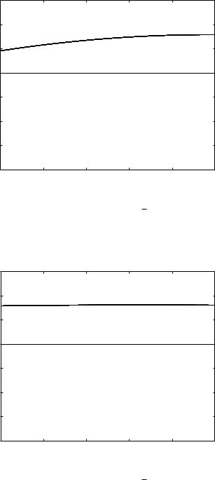
As the ratio of wave length to tube length increases, the pressure distribution changes considerably. Examples are shown in Figs. 8.7.6–9 where

294 8 Elements of Unlumped-Model Analysis

normalized pressure

2.5
2
1.5
1
0.5
0
−0.5
−1
−1.5
−2
−2.50	0.2	0.4	0.6	0.8	1
		normalized distance

Fig. 8.7.4. Wave reflections in a tube when the wave length and the tube length are equal, i.e., λ = 1.0, and the reflection coe cient R = 0.8. The thin lines represent the oscillatory pressure at di erent points in time within the oscillatory cycle, each line representing the sum of the forward and the backward moving waves which are not shown here. The bold line represents the “pressure distribution” along the tube, which is the distribution of peak pressures reached at di erent points along the tube. The distribution in this case is to be compared with that in Fig. 8.7.2 where wave reflections are absent.

normalized pressure

2.5
2
1.5
1
0.5
0
−0.5
−10	0.2	0.4	0.6	0.8	1
		normalized distance

Fig. 8.7.5. Solid line: Pressure distribution along a tube (from Fig. 8.7.4) as modified by wave reflections when the wave length and the tube length are equal (λ = 1.0) and the reflection coe cient R = 0.8. The points of maxima and minima are sometimes referred to as “node points” and in this case are spaced one quarter tube lengths apart. Dashed line: Pressure distribution in the absence of wave reflections.

normalized pressure

				8.7 Wave Reflections		295
2.5
2
1.5
1
0.5
0
−0.5
−10	0.2	0.4	0.6	0.8	1
		normalized distance

Fig. 8.7.6. Solid line: Pressure distribution along a tube as modified by wave reflections when the wave-length-to-tube-length ratio λ = 2 and the reflection coe cient R = 0.8. Dashed line: Pressure distribution in the absence of wave reflections.

normalized pressure

2.5
2
1.5
1
0.5
0
−0.5
−10	0.2	0.4	0.6	0.8	1
		normalized distance

Fig. 8.7.7. Pressure distributions in the presence (solid line) and absence (dashed line) of wave reflections as in Fig. 8.7.6 but here with λ = 5 and R = 0.8.

296 8 Elements of Unlumped-Model Analysis

	2.5
pressure	2
	1.5
normalized	1
	0.5
	0
	−0.5
	−10	0.2	0.4	0.6	0.8	1
			normalized distance

Fig. 8.7.8. Pressure distributions in the presence (solid line) and absence (dashed line) of wave reflections as in Fig. 8.7.6 but here with λ = 10 and R = 0.8.

normalized pressure

2.5
2
1.5
1
0.5
0
−0.5
−10	0.2	0.4	0.6	0.8	1
		normalized distance

Fig. 8.7.9. Pressure distributions in the presence (solid line) and absence (dashed line) of wave reflections as in Fig. 8.7.6 but here with λ = 100 and R = 0.8.

8.8 Summary

297

λ = 2, 5, 10, 100. It is seen that the number of node points is reduced to two at λ = 2 and there are no node points at all for λ > 4. In all cases, the value of the normalized pressure amplitude at the terminal end of the tube (x = 1.0) is 1 + R as prescribed by Eq. 8.7.30. The characteristic pattern of the pressure distribution at higher values of λ is described by a monotonically increasing function, edging closer and closer towards a uniform value of 1 + R as prescribed by Eq. 8.7.33. These higher values of λ are particularly relevant in coronary blood flow where the lengths of main coronary arteries and their branches are of the order of centimeters while the wave length is of the order of meters.

8.8 Summary

In unlumped-model analysis internal structures and events within the coronary circulation are considered, thus introducing a space dimension which does not exist in lumped models. In particular, the intricate vascular structure within the system and flow events within this structure, including wave propagation and wave reflections, provide the main grounds for unlumped-model analysis.

A space dimension is an essential part of unlumped-model analysis, whether for flow in a single vessel segment or flow along the tree structure of coronary vasculature. In both cases flow properties are considered to be functions of space and time. In lumped-model analysis, by contrast, they are considered to be functions of time only.

In a sequence of tube segments in series, assuming idealized Poiseuille flow in each segment, the streamwise distribution of pressure along the tube segments depends critically on their successive diameters. The pressure drops linearly if successive diameters are unchanged, it drops more steeply if successive diameters are decreasing and less steeply if they are increasing.

Arterial bifurcations are the building block from which the tree structure of coronary vasculature is constructed. The pressure distributions in steady Poiseuille flow along the two paths in a bifurcation depend on the power law relation between the diameter of a vessel segment and the flow rate which the vessel is destined to convey. Under the “cube law”, whereby the diameter is proportional to the cube root of the flow rate, the pressure drops linearly and equally along both paths.

Pulsatile flow in a rigid tube may be divided into a steady part and an oscillatory part and, because the equations governing the flow are linear, the two parts can be dealt with separately and the results then simply added. A characteristic feature of oscillatory flow in a rigid tube is that velocity profiles at a particular moment in time are the same at every streamwise position along the tube. In other words, the velocity field is a function of time only, not a function of position along the tube. This is only possible when the tube is rigid, hence the results cannot be applied to coronary vasculature because

298 8 Elements of Unlumped-Model Analysis

of the elasticity of the vessels, but the results and the solutions on which they are based form the basis for a solution for pulsatile flow in an elastic tube.

Pulsatile flow in an elastic tube consists of wave motion along the tube. The velocity field within the tube is a function both of time and of streamwise position along the tube. At a fixed point in time the pressure distribution along the tube is periodic in position, while at a fixed position along the tube the pressure is periodic in time. A key parameter of the flow is the wave speed, which represents the speed with which the wave motion progresses along the tube. Pulsatile flow within coronary vasculature has the characteristics of pulsatile flow in an elastic tube.

One of the most important consequences of wave propagation in an elastic tube is the possibility of wave reflection. Reflections arise when a forward moving wave meets an “obstacle”, a change in the conditions under which it is moving. Part of the wave is reflected, thus giving rise to a backward moving wave and the combination of the two waves changes the pressure distribution within the tube. In coronary blood flow the most common obstacle is a vascular junction, and since there are so many of these within the coronary vasculature, the cumulative e ect of wave reflections can be very large.

9

Basic Unlumped Models

9.1 Introduction

There are as yet no well defined or complete unlumped models of the coronary circulation. Work towards this goal has been going on for some time but the subject is still in its infancy because the first few decades of that work were spent largely on attempts to unravel the functional anatomy of coronary vasculature [94, 69, 16, 127, 61, 73, 196, 133, 182, 81, 227, 228, 223, 224, 214, 229, 216, 106, 218, 175, 233, 39, 103, 181]. Also, studies of flow within this vasculature, whether theoretical or experimental, have been rather sporadic because of the enormous di culties involved, and have so far been able to consider only flow in specific parts of coronary vasculature or only specific aspects of coronary blood flow [108, 38, 11, 12, 160, 101, 143, 88, 104, 159, 170, 219, 105, 109, 18, 144, 148, 99, 23, 231].

The ultimate unlumped model of the coronary circulation would be one in which the branching architecture of coronary vasculature is represented in accurate details, the elasticities and other properties of all vessel segments within the coronary network are specified, intramyocardial pressure is mapped out in space within the myocardium and in time within the oscillatory cycle so that its e ect on flow in each vessel segment at each moment during the oscillatory cycle is determined, regulatory feedback loops and mechanisms are integrated into the dynamics of the system, and the form of the input pressure wave is specified.

It is an unattainable model, and likely an unnecessary luxury even if it could be attained. The representation of every vessel segment within the coronary network in a model of the coronary circulation is not only an (almost) impossible task but also a wasteful one because the detailed architecture of the coronary network is highly variable from one heart to another [228, 216]. Two coronary networks are never the same in terms of the location and properties of every vessel segment. Therefore, to strive for the validity of such details in a model of the coronary circulation is not highly meaningful, even if it were possible.