The Physics of Coronory Blood Flow - M. Zamir

5.6 Example: Cardiac Waveform

169

5.6 Example: Cardiac Waveform

Using the numerical formulation of the previous section and the numerical data in Table 5.1.1 for the cardiac waveform shown in Fig. 5.1.1, we are now in a position to apply Fourier analysis to this wave and to find its harmonics. Essentially, the analysis is the same as for other waves except for the evaluation of the Fourier coe cients An, Bn, which in this case must be done numerically.

For A0, using Eq. 5.5.8 and values from Table 5.1.1, we find
		Δt
A0 =			{p0 + p1 + p2 + . . . + pN −1}			(5.6.1)
		N
=	0.025			{−7.7183 − 8.2383	− 8.6444 + . . . − 6.8024}	(5.6.2)
		40
=	0.025 × 0.00000475					(5.6.3)
≈	0					(5.6.4)

We recall from previous examples that A0 represents the average value of the periodic function p(t) over one complete period. Thus, the fact that this average value is zero in this case indicates that the waveform in Fig. 5.1.2 represents only the oscillatory part of a cardiac wave, any constant part has been removed. It is always possible, and in fact desirable, to remove any constant average from a waveform before applying Fourier analysis to it because the analysis is concerned with only the oscillatory part. This principle is illustrated graphically in Fig. 5.6.1.

For the other Fourier coe cients, using Eqs.5.5.12,16 and the data in Table 5.1.1, and noting that the number of data points N = 40 and the period

T = 1.0, we find	= N p0 cos				+ p1 cos			+ . . .
An			T	0		T	1
	2		2nπt			2nπt

+ pN −1 cos	2nπtN −1	Δt	(5.6.5)
	T

=201 {−7.7183 × cos (2nπ × 0) −8.2383 × cos (2nπ × 0.025) + . . .

−6.8024 × cos (2nπ × 0.975)} × 0.025								(5.6.6)
Bn = N p0 sin		T	0	+ p1 sin	T	1		+ . . .
2		2nπt			2nπt

	+ pN −1 sin				2nπtN −1	Δt	(5.6.7)
					T
=	1		{−7.7183		× sin (2nπ × 0)
		20
		−8.2383		× sin (2nπ × 0.025) + . . .
	−6.8024			× sin (2nπ × 0.975)} × 0.025			(5.6.8)

170 5 The Analysis of Composite Waveforms

	140
	120
	100
	80
magnitude	60
	40
	20
	0
	−20
	0	0.5	1
		time

Fig. 5.6.1. A cardiac wave such as the solid curve at the top can always be separated into a purely constant part and a purely oscillatory part. The purely oscillatory part is shown at the bottom and it has the property that its average over one period is zero. In Fourier analysis the constant part of the wave is represented by A0, thus the result A0 = 0 in Eq. 5.6.3 indicates that the data on which the result is based represents only the oscillatory part of the waveform, any constant part has been removed.

We recall that values of n in these expressions refer to di erent harmonics. Thus, evaluating these for the first 10 harmonics (n = 1, 2, . . . , 10), the results are shown numerically in Table 5.6.1.

The Fourier representation of this waveform, using the compact form in Eqs.5.2.21,22, is given by

p(t) = A0	+ n=0 Mn cos			2 T	− φn			(5.6.9)
	∞			nπt
			2T		+ M2 cos	T
= A0	+ M1 cos			− φ1			− φ2
			πt			4πt

+M3 cos	6πt	− φ3	+ ...	(5.6.10)
	T

5.6 Example: Cardiac Waveform

171

Table 5.6.1. Values of the Fourier coe cients for the cardiac wave shown in Fig. 5.6.1, using Eqs.5.6.5,7 with n = 1, 2 . . . 10.

n	An	Bn	Mn	φn (deg)
1	-7.98840	0.15707	7.99000	178.8736
2	-0.42846	-4.41890	4.43960	-95.5381
3	0.88370	0.46246	0.99740	27.6238
4	0.68508	0.28468	0.74187	22.5649
5	-0.35969	0.87460	0.94567	112.3553
6	-0.30961	-0.28316	0.41956 -137.5548
7	-0.53143	-0.20924	0.57114 -158.5089
8	0.26366	-0.15171	0.30419	-29.9153
9	0.02955	0.06432	0.07078	65.3256
10	0.04842	0.16564	0.17258	73.7050

Thus, using values of Mn and φn from Table 5.6.1, the first 10 harmonics of this waveform are given by, recalling that T = 1.0,

p1(t) = M1 cos		2πt			− φ1													(5.6.11)
		T
= 7.99 × cos 2πt −							178.		8736		×	π
																		(5.6.12)
									180
p2(t) = M2 cos		4πt			− φ2													(5.6.13)
		T
									5381						π
= 4.4396 × cos 4πt −								−95.				×						(5.6.14)
								180
.
.
.
p10(t) = M10 cos			20πt			− φ10												(5.6.15)
			T
									705					π
= 0.17258 × cos 20πt −										73. ×								(5.6.16)
										180

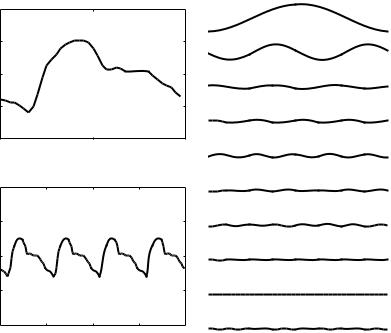
Using these results, the cardiac waveform and its first 10 harmonics are shown in Fig. 5.6.2.

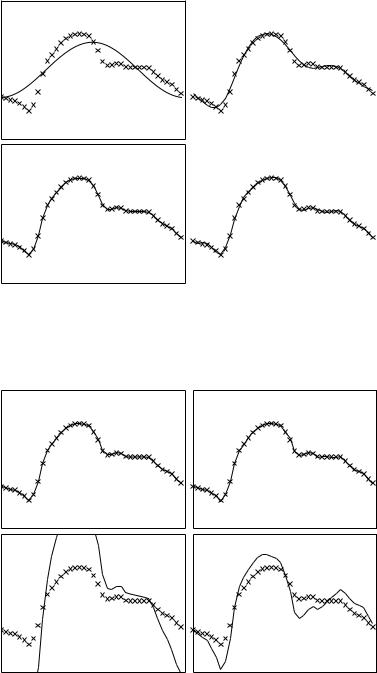
Fig. 5.6.3 shows the accuracy of this Fourier representation of the cardiac waveform when only the first one, four, seven, and ten harmonics are used. It is seen that the representation is fairly accurate with only the first seven harmonics. By contrast, Fourier representations of the single-step and the piecewise waveforms considered in the previous sections were less accurate with as many as fifty harmonics. The reasons for this can be seen clearly in Figs.5.3.3 and 5.4.4. The presence of step changes in those cases, and the behaviour of the Fourier curves in the vicinity of these steps, shows that Fourier

172 5 The Analysis of Composite Waveforms

20
10
0
−10
−20		0.5		1
0
40
20
0
−20
−40	1	2	3	4
0

Fig. 5.6.2. The cardiac waveform of Fig. 5.1.1 with its first ten harmonics, using the results in Eqs.5.6.10-15.

series have di culty replicating step changes. The cardiac waveform does not contain such changes, thus higher accuracy is achieved with a relatively small number of harmonics.

In fact, as mentioned earlier, when the waveform to be represented by a Fourier series is available only in numerical form, the number of harmonics that produces the most accurate representation becomes dependent on the number of data points available in the numerical description of the waveform. Broadly speaking, the theory of Fourier analysis has shown that if the number of data points available is N , then the number of harmonics that produces the most accurate representation is N/2 [28, 197]. A smaller or a larger number of harmonics produce a less accurate representation, for di erent reasons. This is an oversimplification of the underlying theory, but it provides a useful guide, indeed a necessary guide, for practical applications of Fourier analysis to specific waveforms.

For the cardiac waveform being considered in this section, the number of data points in the numerical description of the wave (Table 5.1.1) is 40, thus the number of harmonics required to produce the most accurate representation is 20. However, it turns out that this maximum accuracy is reached along a fairly shallow (not sharp) peak, thus the optimum number of harmonics

5.6 Example: Cardiac Waveform	173

Fig. 5.6.3. Fourier series representations of the cardiac waveform, based on the first one, four, seven, and ten harmonics, clockwise from top left corner.

Fig. 5.6.4. Fourier series representation of the cardiac waveform, based on the first 20, 30, 38, and 45 harmonics, clockwise from top left corner.

174 5 The Analysis of Composite Waveforms

	20
	15
	10
magnitude	5
	0
	−5
	−10
	−15
	−200	0.2	0.4	0.6	0.8	1
				time

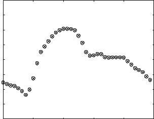
Fig. 5.6.5. Fourier series representation of the cardiac waveform based on a Fast Fourier Transform (FFT) program, where crosses represent the original data points describing the waveform and circles represent the corresponding data points produce by the Fourier series representation. The program precisely replicates the original data points.

need not be treated precisely. In other words, 19 or 21 harmonics will not produce significant di erences. In fact, as seen in Fig. 5.6.3, both seven and ten harmonics produce fairly accurate representations, and the di erence between them is barely detectable. A Fourier representation with precisely 20 harmonics is shown in Fig. 5.6.4, compared with representations using 30, 38, and 45 harmonics. It is seen that only in the latter two cases the representation breaks down. A representation based on a Fast Fourier Transform (FFT) program is shown in Fig. 5.6.5, where it is seen that the program can produce precisely the data points given in the numerical description of the waveform.

5.7 Summary

The driving pressure in the dynamics of the coronary circulation has a composite waveform such as the cardiac pressure wave, while much of the analysis described so far deals with only simple sine or cosine waves. The theory of Fourier analysis shows that a composite wave can in fact be expressed as the sum of a series of sine and cosine waves which are referred to as its “harmonics”. This makes it possible to extend lumped model analysis, which is based on only simple sine and cosine waves, to now include composite pressure and flow waveforms.

5.7 Summary

175

A composite wave is a periodic function of time with period T and angular frequency ω. Its harmonics can be expressed as cosine functions, the first has a period T and angular frequency ω and is referred to as the “fundamental harmonic”, the second has a period T /2 and angular frequency 2ω, and so on. In many cases the first 10 harmonics are su cient for producing a good representation of a given periodic function such as the composite pressure wave produced by the heart. In that case, the fundamental frequency is the beating frequency of the heart which, under resting conditions, is approximately 1 Hz, thus the frequency of the tenth harmonic would be 10 Hz. It is for this reason that frequencies as high as 10 Hz are considered in the dynamics of the coronary circulation and of the cardiovascular system in general.

A very simple example of a composite waveform is a single step that is repeated continuously with a period T . The example illustrates how the shape of the step is gradually approximated as more and more harmonics are added.

Another example of a composite waveform is a “piecewise” form consisting of several steps. Fourier analysis of the waveform is essentially the same as for the single-step waveform, but the example illustrates how the Fourier series approximation has di culties at sharp corners.

Composite waveforms of interest in the dynamics of the coronary circulation, such as the cardiac pressure waveform, can only be expressed in numerical form. A numerical formulation of Fourier analysis makes it possible to use the numerical form of the composite wave and proceed to find its harmonics as for other waves.

Typically, 40 data points would normally be su cient to represent a cardiac waveform numerically. The number of harmonics that produces the most accurate Fourier series representation of the waveform is then 20. A smaller or larger number of harmonics produces a less accurate representation. Fourier series replicate the cardiac waveform more easily than they do a piecewise waveform because of the absence of sharp steps in the former.

6

Composite Pressure-Flow Relations

6.1 Introduction

As stated earlier in this book, in the overwhelming majority of heart failures the precipitating factor is a lack of blood supply to the heart itself for its own metabolic needs [83, 206, 14, 128]. In other words, in most cases of what is generally referred to as “heart disease”, the heart is not truly diseased in the normal sense of the word, it is simply being deprived of the energy it needs to do its work. And the work of the heart is important, of course, because it is the pump that provides blood supply to all other parts of the body.

As described in Chapter 1, blood supply to the heart, or coronary blood flow, comes via two branches of the aorta as shown in Figs. 1.3.1, 2. Many factors and mechanisms are involved in the short journey of blood from this point at the base of the aorta to points within the myocardium. The one that attracts most attention in medical practice is obstruction of the blood vessels. However, the journey of coronary blood flow involves some of the most complex and highly delicate dynamics and control mechanisms. They can equally disrupt blood supply to the heart. In this chapter and in this book in general, the focus is on these dynamic aspects of coronary blood flow.

The dynamics and control mechanisms of coronary blood flow require as much attention as the obstruction of blood vessels not only because they can and do interfere with orderly blood supply to the heart but because these dynamic aspects of coronary blood flow are not fully known or fully understood and are far less “visible” than an obstruction of a blood vessel. We have seen even in the crude models discussed in previous sections that, because of the pulsatile nature of coronary blood flow, any change that a ects capacitance or inductance within the coronary circulation can have significant e ects on the dynamics of coronary blood flow. The change may come about as a result of pathology, injury, or the administration of drugs or surgery that alter the properties of the conducting vessels or of the moving fluid. Any of these can disrupt the delicate dynamic balance of the system and thus disrupt blood supply to heart tissue.

178 6 Composite Pressure-Flow Relations

Much of the dynamics of coronary blood flow is “hidden” in the sense that many elements of these dynamics cannot be easily measured. Not only are the controlling parameters such as capacitance and resistance inaccessible to direct measurement but direct measurements of pressure and flow which these parameters control are extremely di cult because of the small size of the vessels involved, the violent pulsations of the living heart, and the phase di erence between pressure and flow which necessitates simultaneous measurements of both for any meaningful interpretation.

An element of the dynamics of the coronary circulation that is reasonably accessible is the pressure at the base of the aorta or at the entrances to the two main coronary arteries (Fig. 1.3.2). This pressure provides an important key into the coronary circulation because it represents the force that drives flow into the coronary system. It is the external force in the forced dynamics scenarios of the RLC systems examined in Chapter 4. While the driving force is actually the di erence between this pressure and pressure at exit from the system at the capillary level, it is reasonable to neglect the small pressure at exit and think of the pressure at entry into the system as the driving pressure drop. Thus, if this pressure is denoted by P (t), in this chapter we shall use the notation P (t) for the pressure drop driving the flow, instead of Δp used in Chapter 4. This is convenient not only because it simplifies the notation in this chapter but because this pressure represents the pressure wave generated by the heart as it just emerges from the left ventricle, and measurements of this pressure are widely available. We shall refer to it simply as the “cardiac pressure wave”.

With the cardiac pressure wave P (t) taken as the force driving coronary blood flow, the ultimate aim of all modelling and experimental studies is to determine the corresponding flow wave generated by this force, which we shall denote by Q(t). In experimental studies, because of lack of access and other di culties, Q(t) would most likely represent inflow, that is flow at entry into the system. It would be measured at the same location as P (t), at the base of the aorta as flow enters the two main coronary ostia, or somewhere further downstream along the two main coronary arteries. In modelling studies, depending on whether the system is being modelled by a parallel or a series circuit, Q(t) may be broken down into inflow and outflow, if they di er, or into partial flows along di erent branches of the parallel circuit. In physiological or clinical studies, of course, the ultimate question is how much blood flow is reaching the myocardium, therefore one would like Q(t) to represent outflow from the system.

It must be remembered that both P (t) and Q(t) are functions of time, periodic functions of time, each in general being represented by a composite waveform. Thus, the relation between pressure and flow is itself a function of time, it is di erent at di erent points in time within the oscillatory cycle. Only when P (t) is a simple sine or cosine function, that is, when it is a single harmonic, does the relation between pressure and flow remain the same during the oscillatory cycle and Q(t) can be described simply by a fixed

6.2 Composite Pressure-Flow Relations Under Pure Resistance

179

amplitude and a fixed phase angle as was done in previous sections. In that case, a fixed relation exists between the amplitudes and phase angles of the pressure and flow waves. When P (t) is a composite waveform, however, Q(t) is also a composite waveform and no such simple relation between the two is possible because the two composite waves cannot be described in terms of single amplitudes and phase angles. But, as we saw in the previous chapter, the two waves can be decomposed into harmonics which can be described in this simple way and, as we shall see in this chapter, the simple relation between pressure and flow continues to apply to the harmonics of the composite pressure and flow waves.

It must be remembered, also, that the relations between the harmonics of pressure and flow waves, namely the relations based on the concept of impedance introduced in Section 4.9, represent only steady state dynamics, not including any transient e ects as discussed in Section 4.7. This is not an unreasonable modelling strategy of the coronary circulation because the normal operating mode of the system is that of steady state oscillation, and because a good understanding of the dynamics of the system must be based on this normal steady state mode. Indeed, steady state dynamics form the basis of all lumped models of the coronary circulation, and they form the basis of the pressure-flow relations to be explored in this chapter.

The ultimate aim then is a relation between the form of the composite pressure wave P (t) and the form of the corresponding flow wave Q(t). In medical practice the form of the cardiac pressure wave is highly scrutinized in terms of its graphic details, mainly because these details are interpreted as indicators of the enegertic performance of the cardiac muscle. Yet, this same pressure waveform is responsible for driving coronary blood flow, and its graphic details can equally be interpreted as indicators of the amount of flow going into the coronary circulation. Such interpretation requires an understanding of the relation between the two composite waveforms, however, and this is the subject of the present chapter.

6.2Composite Pressure-Flow Relations Under Pure Resistance

In this section we consider the relation between a composite pressure waveform and the corresponding flow waveform when the opposition to flow consists of only pure resistance. While, as we shall see, this is a rather trivial case, it provides a good starting point and an important reference for subsequent cases. It also serves to illustrate the analytical steps required to obtain the composite flow waveform Q(t) from a given composite pressure waveform P (t).

We recall that when P (t) is a simple sine or cosine function, as in Eq. 4.8.2,

P (t) = P0 cos ωt

(6.2.1)