The Physics of Coronory Blood Flow - M. Zamir

200 6 Composite Pressure-Flow Relations

pn(t)

qnr (t) = (6.6.7)

Zn

=

pnr + ipni

(6.6.8)

znr + izni

=

pnr znr + pnizni

(6.6.9)

z2

+ z2

nr

ni

2

2πnt

2πnt

= R(ωnC) Mn cos

T

1 + ( n

T

− φn

− ωnCMn sin

− φn

Rω C)2

(6.6.10)

and for the corresponding harmonics of the R-scaled flow wave

×

2

2πnt

1 + (

n C

2πnt

(ωntC ) Mn cos

T

T

R

qnr (t) =

− φn

−

ωntC Mn sin

− φn

ω t

)2

(6.6.11)

where tC is the inertial time constant, given by

tC = RC

(6.6.12)

We recall from Section 2.6 that C and tC are measures of the compliance of the vascular system or the balloon used as a model. The higher the value of C or tC , the more compliant the system is, allowing a greater change in its volume and hence more flow into it. This factor is extremely important in the coronary circulation because it intervenes between flow entering the system at the root of the main coronary arteries and flow leaving the system at the capillary end. In the absence of compliance the two flows would be equal at all times, thus a measurement of flow at entry gives a measure of the flow being delivered at the all-important receiving end. In the presence of compliance, the connection between inflow and outflow is lost, and while over one or more oscillatory cycles the two flows will normally be equal, at any one moment within an oscillatory cycle they are unequal.

Thus, a good model of the role of capacitance in the dynamics of the coronary circulation is essential, and much of the research work in this area has been directed at this problem. In particular, e orts have been directed at obtaining an estimate of the value of the capacitance C. From the definition of C in Section 2.6 (Eq. 2.6.6), the dimensions of C are seen to be the dimensions of volume over pressure which indeed represents the change in volume obtained from a given change in pressure. The higher the value of C the higher the change in volume obtained for a given change in pressure, and hence the more “compliant” the system is. In a series of experiments by Judd et al [97, 98] it was estimated that for the dog heart the value is 0.002 ml/mm Hg per 100 g of heart tissue. If, for the purpose of discussion we consider the dog’s heart to

6.6 Composite Pressure-Flow Relations Under Capacitance E ects

201

actually be 100 g (= 0.5% of body weight), then the value of C for the entire coronary system of that dog is 0.002 ml/mm Hg.

Consistent with previous chapters, in what follows we shall continue to use the capacitive time constant tC as a measure of capacitance or compliance, rather than C. The dimensions of tC are, of course, the dimensions of time, and we shall use seconds for the units of tC as we did for the inertial time constant tL. Using the above estimate for C, and the estimate for the resistance R obtained in Section 6.3 for the coronary system of a 20 kg dog, (Eq. 6.3.12), we find tC ≈ 0.12 s for that system. We shall use this value as a guide to the range of values of tC used in what follows.

With the individual harmonics of the oscillatory part of the R-scaled flow wave obtained from Eq. 6.6.11, the complete oscillatory flow wave is finally

obtained by adding these harmonics, that is
R × qr (t) = R × q1r (t) + R × q2r (t) . . . + R × qN r (t)	(6.6.13)

where N is the number of harmonics. The complete R-scaled flow wave (corresponding to real part of driving pressure) is then given by

R × Q(t) = R ×		+ R × qr (t)	(6.6.14)
	q

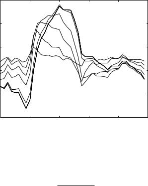
Results, comparing the R-scaled flow wave with the corresponding pressure wave at di erent values of tC , and using the one-step, piecewise, and cardiac pressure waves, are shown in Fig. 6.6.1–3. It is seen that when tC is high, indicating high compliance, the R-scaled flow curve comes close to the pressure curve. Recalling that here the resistance and capacitance are in series, the result indicates that the capacitor is not having much e ect on the flow rate, the latter being close to what it would be in the absence of the capacitor. By contrast, when tC is low, which corresponds to low compliance, the R-scaled flow rate is reduced to almost steady flow at the average value of the driving pressure. The capacitor in this case has a considerable e ect on the flow. It is, e ectively, damping the oscillatory part of the flow.

When resistance and capacitance are in parallel, the complex impedance, from Eqs. 4.9.33, 34, 36 and in the notation of the present section, is given by

	1	=		1	+ iωnC		(6.6.15)
	Zn			R
so that
Zn =					R		(6.6.16)
			1	+ iRωnC
=			R − iωnCR2				(6.6.17)
			1	+ (RωnC)2

and the real and imaginary parts of the complex impedance are thus given by

202 6 Composite Pressure-Flow Relations

	1.5
(mmHg)	1		a
flow		b
		c
R−scaled	0.5	d
		e
pressure,	0
	−0.50	0.2	0.4	0.6	0.8	1
			time t (normalized)

Fig. 6.6.1. Pressure (solid) and R-scaled flow waves (dashed) through a resistance R and capacitance C in series, and for di erent values of the capacitive time constant tC in seconds: (a) 1.0, (b) 0.2, (c) 0.1, (d) 0.04, (e) 0.01. At the highest value of tC the R-scaled flow curve is closest to the pressure curve, indicating that the capacitor is not having much e ect on the flow rate, the latter being close to what it would be in the absence of the capacitor. When tC is low, by contrast, the R-scaled flow rate is reduced to almost steady flow at the average value of the driving pressure. The capacitor in this case is e ectively damping the oscillatory part of the flow.

	1.5
(mmHg)	1		a
flow
			b
			c
R−scaled	0.5	d
		e
pressure,	0
	−0.50	0.2	0.4	0.6	0.8	1
			time t (normalized)

Fig. 6.6.2. See caption for Fig. 6.6.1.

6.6 Composite Pressure-Flow Relations Under Capacitance E ects

203

	115
flow (mmHg)				a
	110		b
			c
	105		d
R−scaled			e
	100
pressure,	95
	900	0.2	0.4	0.6	0.8	1
			time t (normalized)

Fig. 6.6.3. See caption for Fig. 6.6.1.

	znr =		R	(6.6.18)
		1	+ (RωnC)2
	zni =		−ωnCR2	(6.6.19)
		1	+ (RωnC)2

Following the same steps as in the previous section, the R-scaled flow wave is given by

R × qnr (t) = Mn cos	T	− φn − ωntC Mn sin		2 T − φn
	2πnt			πnt

(6.6.20)

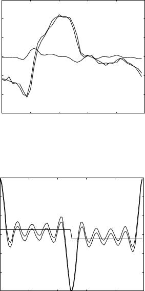
Results for a low value of the capacitance time constant (tC = 0.01 s) are presented in Figs. 6.6.4–6 where R-scaled total flow and R-scaled capacitive flow are shown separately. In this case, because of the low value of tC , which indicates low compliance, and because the capacitance is in parallel with the resistance, most flow is through the resistor with very little flow going through the capacitor. The situation is the reverse of that in Figs. 6.6.1–3 where the resistance and capacitance are in series.

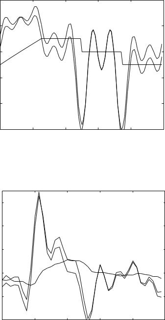
Results for a high value of the capacitive time constant (tC = 0.3) are shown in Figs. 6.6.7–9. In this case, because of the high compliance within the system, and because this compliance is in parallel with the resistance, very high flow rates are drawn into the capacitor and very little (by comparison) into the resistor. R-scaled total flow waveform is very far from the pressure waveform, consistent with large capacitive e ects.

204 6 Composite Pressure-Flow Relations

	0.8
(mmHg)	0.6
	0.4
flow	0.2
R−scaled	0
	−0.2
pressure,	−0.4
	−0.6
	−0.80	0.2	0.4	0.6	0.8	1
			time t (normalized)

Fig. 6.6.4. R-scaled total flow (dashed) and R-scaled capacitive flow (dotted) through a resistance and capacitance in parallel and under the driving composite pressure wave shown by the solid curve and with a low value of the capacitive time constant (tC = 0.01). Because of low compliance, capacitive flow is near zero, hence total flow is mostly through the resistor as indicated by the closeness of the total flow and pressure curves.

	0.6
(mmHg)	0.4
	0.2
flow	0
R−scaled
	−0.2
pressure,	−0.4
	−0.6
	−0.80	0.2	0.4	0.6	0.8	1
			time t (normalized)

Fig. 6.6.5. See caption for Fig. 6.6.4.

6.6 Composite Pressure-Flow Relations Under Capacitance E ects

205

	15
(mmHg)	10
	5
flow
R−scaled	0
	−5
pressure,
	−10
	−150	0.2	0.4	0.6	0.8	1
			time t (normalized)

Fig. 6.6.6. See caption for Fig. 6.6.4.

	6
(mmHg)	4
	2
flow
R−scaled	0
	−2
pressure,
	−4
	−60	0.2	0.4	0.6	0.8	1
			time t (normalized)

Fig. 6.6.7. R-scaled total flow (dashed) and R-scaled capacitive flow (dotted) through a resistance and capacitance in parallel and under the driving composite pressure wave shown by the solid curve and with a high value of the capacitive time constant (tC = 0.3). Because of the high compliance, very high flow rates are drawn into the capacitor, with very little (by comparison) drawn into the resistor. Pressure and total flow waveforms are far apart, consistent with large capacitive e ects.

206 6 Composite Pressure-Flow Relations

	2
flow (mmHg)	1
	0
R−scaled
	−1
pressure,	−2
	−30	0.2	0.4	0.6	0.8	1
			time t (normalized)

Fig. 6.6.8. See caption for Fig. 6.6.7.

flow (mmHg)	60
	40
R−scaled	20
	0
pressure,
	−20
	−400	0.2	0.4	0.6	0.8	1
			time t (normalized)

Fig. 6.6.9. See caption for Fig. 6.6.7.

6.7 Composite Pressure-Flow Relations Under RLC in Series

207

6.7Composite Pressure-Flow Relations Under RLC in Series

The RLC system in series provides a basic model in which the elements of resistance, inductance, and capacitance are all present but their e ects are constrained by each other because of their series arrangement. Free and forced dynamics of this system have been examined in previous chapters using zero, linear, or sinusoidal driving pressures. In this section we examine pressure flow relations under this system, using composite driving pressure waves.

The complex impedance for R, L, C in series was found in Section 4.9, Eq. 4.9.41, namely

	1
Z = R + i ωL −	ωC	(6.7.1)

where ω is the angular frequency of oscillation of the driving pressure. For a composite pressure wave consisting of N harmonics the impedance will be di erent for each of these harmonics because of their di erent frequencies, and we shall use the notation

		1		(6.7.2)
Z = R + i	ωnL −	ωnC
ωn = 2πn	n = 1, 2, . . . , N			(6.7.3)

where n denotes a particular harmonic and ωn is the angular frequency of that harmonic. For the real and imaginary parts of the impedance, using subscripts r, i as before, we have in this case

znr = R		(6.7.4)
zni = ωnL −	1	(6.7.5)
	ωnC

In the notation of previous sections, consider the composite pressure wave

P (t) =

p

+ p(t)

(6.7.6)

where p is the mean value of P (t) over one oscillatory cycle, which is also referred to as the “steady part” of P (t), and p(t) is the purely oscillatory part of P (t), meaning, as we saw earlier, that the mean value of p(t) over one oscillatory cycle is zero. Being generally a composite wave, this part of the driving pressure wave is represented in terms of its harmonics which we shall denote by pn(t), where n = 1, 2, . . . , N and N is the total number of harmonics used in that representation. It was seen in Chapter 5 that for any composite waveform these harmonics can be put in the form

pn(t) = Mn cos (ωnt − φn) n = 1, 2, . . . , N

(6.7.7)

208 6 Composite Pressure-Flow Relations

where Mn are the Fourier coe cients and φn the phase angles discussed in Chapter 5, and where time t has been normalized such that the oscillatory cycle is in the interval t = 0 to t = 1, which is equivalent to taking the period of oscillation T = 1. We shall use this normalization throughout this chapter. Furthermore, the pressure-flow analysis is greatly simplified if the harmonics in Eq. 6.7.7 are seen as the real parts of the corresponding complex set of harmonics, namely

pn(t) = pnr (t)			(6.7.8)
pnr (t) = Mnei(ωn t−φn )			(6.7.9)
= Mn cos (ωnt − φn)		n = 1, 2, . . . , N	(6.7.10)

The corresponding imaginary parts of these harmonics, which are required in the analysis below, are then given by

pni(t) =	Mnei(ωn t−φn )	(6.7.11)
= Mn sin (ωnt − φn) n = 1, 2, . . . , N		(6.7.12)

The advantage of using the complex form of the harmonics of the pressure wave is that it makes the relation between these and the corresponding harmonics of the flow wave particularly simple, namely

	complex flow harmonic =	complex pressure harmonic		(6.7.13)
		Zn

and since the driving pressure wave in this presentation is composed of the real parts of the complex pressure harmonics (Eq. 6.7.9), the resulting flow wave is composed of the real parts of the complex flow harmonics, that is

qnr (t) =

Mne

i(ωn t

−

φn )

(6.7.14)

Zn

=

pnr znr + pnizni

(6.7.15)

z2 + z2

nr

ni

RMn cos (ωnt − φn) +

1

Mn sin (ωnt − φn)

ωnL −

=

ωn C

(6.7.16)

R2 +

ωnL − ωn C

2

1

and the corresponding R-scaled flow harmonics are

		1
R × qnr (t) =	Mn cos (ωnt − φn) + ωntL −	ωn tC		Mn sin (ωnt − φn)	(6.7.17)
	1 + ωntL −	1		2
		ωn tC

where tL (= L/R) and tC (= CR) are the inertial and capacitive time constants. Both constants are involved in this case because both inertial and

6.7 Composite Pressure-Flow Relations Under RLC in Series

209

capacitive e ects are present. The complete R-scaled oscillatory flow wave is finally obtained by adding its individual harmonics, that is

R × qr (t) = R × q1r (t) + R × q2r (t) . . . + R × qN r (t)

(6.7.18)

and the complete R-scaled flow wave (corresponding to real part of driving pressure) is finally given by

R × Q(t) = R ×		+ R × qr (t)	(6.7.19)
	q

where q is the steady part of the flow wave corresponding to the steady part of the pressure wave p, if any, the two being related by

		=			p		(6.7.20)
	q
			R

Results, comparing the R-scaled flow wave with the corresponding pressure wave, with tL = 0.1 s and a range of values of tC , and using the one-step, piecewise, and cardiac pressure waves, are shown in Fig. 6.7.1–3. They demonstrate that at the highest value of tC the flow wave exhibits a behaviour similar to that of the overdamped dynamics of the LRC system observed in Sections 3.3 and 4.4–6. It must be remembered, however, that overdamped or underdamped conditions relate to the dynamics of the RLC system in the transient

(mmHg)	1.2
	1		a
	0.8		b
flow		c
	0.6	d
R−scaled
	0.4	e
pressure,	0.2
	0
	−0.2
	0	0.2	0.4	0.6	0.8	1
			time t (normalized)

Fig. 6.7.1. Pressure (solid) and R-scaled flow waves (dashed) through the RLC system in series, with the inertial time constant tL = 0.1 s and di erent values of the capacitive time constant tC in seconds: (a) 5.0, (b) 0.2, (c) 0.1, (d) 0.04, (e) 0.01. The highest value of tC corresponds to low compliance (more rigid balloon) and hence flow is dominated by inertial e ects, and at low values of tC the reverse is true.