The Physics of Coronory Blood Flow - M. Zamir

210 6 Composite Pressure-Flow Relations

(mmHg)	1
				a
	0.8			b
flow			c
	0.6		d
R−scaled
			e
	0.4
pressure,	0.2
	0
	−0.20	0.2	0.4	0.6	0.8	1
			time t (normalized)

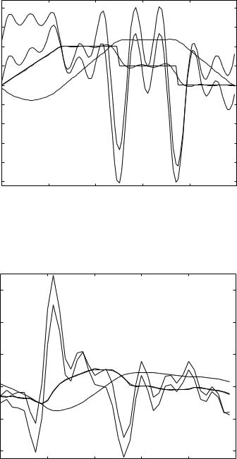
Fig. 6.7.2. See caption for Fig. 6.7.1.

	115
(mmHg)				b
	110
				c
flow
				a
	105		d
R−scaled
	100		e
pressure,	95
	900	0.2	0.4	0.6	0.8	1
			time t (normalized)

Fig. 6.7.3. See caption for Fig. 6.7.1.

6.7 Composite Pressure-Flow Relations Under RLC in Series

211

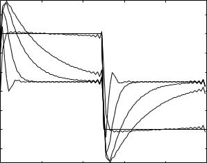
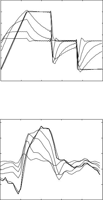
state only, while the results in this section and in the context of lumped models in general relate to the system in steady state only. Nevertheless, the mechanisms underlying the di erent behaviour observed in Figs. 6.7.1, 2 are similar to those underlying overdamped and underdamped behaviour. Here, at the highest value of tC , which indicates low compliance (or a more rigid balloon), the balloon filling occurs without a recoil or oscillations, while at lower values of tC , because of higher compliance of the balloon, the reverse is true. This phenomenon is seen more clearly in Figs. 6.7.1, 2 because the composite pressure waves in these two figures contain step changes in pressure. It is as if these step changes create “micro transient states” within the oscillatory cycle. In Fig. 6.7.3 this does not occur as distinctly because there are no step changes in pressure, although here too, the curve with the highest value of tC is the one with the least oscillations.

Another way of looking at the results in Figs. 6.7.1–3, is that at higher values of tC capacitance e ects are small and the dynamics of the system are dominated by inertial e ects, so that the results resemble those of resistance and inertial e ects in series observed in Section 6.5. At lower values of tC capacitive e ects become more significant to the point of dominating the dynamics, and the results then resemble those of resistance and capacitance e ects in series observed in Section 6.6. In that section, however, inertial effects were entirely absent while Figs. 6.7.1–3 still contain inertial e ects, with

(mmHg)	1.2
	1		a
	0.8
flow			b
		c
	0.6
R−scaled		d
	0.4	e
pressure,	0.2
	0
	−0.2
	0	0.2	0.4	0.6	0.8	1
			time t (normalized)

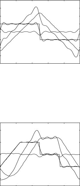
Fig. 6.7.4. Pressure (solid) and R-scaled flow waves (dashed) through the RLC system in series, as in Figs. 6.7.1–3 but with the inertial time constant tL = 0.01 s. This change reduces the inertial e ects to an insignificant level, making the system resemble that of resistance and capacitance in series considered in Section 6.6 and seen in Figs. 6.6.1–3.

212 6 Composite Pressure-Flow Relations

(mmHg)	1			a
	0.8		b
flow			c
	0.6		d
R−scaled
		e
	0.4
pressure,	0.2
	0
	−0.20	0.2	0.4	0.6	0.8	1
			time t (normalized)

Fig. 6.7.5. See caption for Fig. 6.7.4.

	115
(mmHg)				a
	110		b
			c
flow
	105		d
R−scaled
			e
	100
pressure,	95
	900	0.2	0.4	0.6	0.8	1
			time t (normalized)

Fig. 6.7.6. See caption for Fig. 6.7.4.

6.8 Composite Pressure-Flow Relations Under RLC in Parallel

213

tL = 0.1 s. To make the two situations more comparable we must reduce the inertial e ect yet further. Indeed, Figs. 6.7.4–6 show results with the same values of tC as in Figs. 6.7.1–3 but with tL = 0.01 . The flow waves now closely resemble those in Section 6.6, Figs. 6.6.1–3.

6.8Composite Pressure-Flow Relations Under RLC in Parallel

The RLC system in parallel again provides a model in which the elements of resistance, inductance, and capacitance, are all present, but here their e ects are independent of each other because of their parallel arrangement. However, while flow through each element is not a ected by the other two elements, total flow through the system is of course a ected by all three, thus each element continues to a ect total pressure-flow relation. Again, while free and forced dynamics of this system have been examined in previous chapters using zero, linear, or sinusoidal driving pressures, in this section we examine pressure flow relations using composite waves.

The complex impedance for R, L, C in parallel was found in Section 4.9, Eq. 4.9.44, namely

1

1

1

Z

=

R

+ i

ωC −

ωL

(6.8.1)

so that

1 + R

Z =

R − iR2

ωC − ωL1

(6.8.2)

2

2

ωC

−

1

ωL

where ω is the angular frequency of oscillation of the driving pressure. For a composite pressure wave consisting of N harmonics the impedance will be di erent for each of these harmonics because of their di erent frequencies, and we shall use the notation

	R − iR	2			1
Zn =			ωnC −		ωn L					(6.8.3)
	1 + R2	ωnC − ωn L						2
					1
ωn = 2πn			n = 1, 2, . . . , N							(6.8.4)

where n denotes a particular harmonic and ωn is the angular frequency of that harmonic. For the real and imaginary parts of the impedance, using subscripts r, i as before, we have in this case

214 6 Composite Pressure-Flow Relations

znr =			R							(6.8.5)
	1 + R2 ωnC −				1				2
					ωn L
	−R	2		1
zni =			ωnC −	ωn L						(6.8.6)
	1 + R2 ωnC − ωn L								2
					1

Following the same steps as in the previous section, and omitting some of the details, we find the harmonics of the oscillatory flow wave

qnr (t) = Mne				Zn	−	φn )
				i(ωn t
= pnr znr + pnizni
	z2		+ z2
		nr		ni					ωnC − ωn L Mn sin (ωnt − φn)
= Mn cos (ωnt − φn) − R
									1

R

the corresponding R-scaled flow harmonics

R × qnr (t) = Mn cos (ωnt − φn)

−	ωntC −	1	Mn sin (ωnt − φn)
		ωntL

and the complete R-scaled oscillatory flow wave

R × qr (t) = R × q1r (t) + R × q2r (t) . . . + R × qN r (t)

(6.8.7)

(6.8.8)

(6.8.9)

(6.8.10)

(6.8.11)

using the same notation as in the previous section.

Results, comparing the R-scaled flow wave with the corresponding pressure wave, taking tL = 0.1 s and tC = 0.01 s, and using the one-step, piecewise, and cardiac pressure waves, are shown in Fig. 6.8.1–3. Also shown separately in these figures are the R-scaled resistive, inductive, and capacitive flows, which we shall denote by qres(t), qind(t), qcap(t), respectively, and which together make up the total flow wave, that is,

q(t) = qres(t) + qind(t) + qcap(t)

(6.8.12)

Since these three elements of the flow are in parallel in this case, their harmonics, to be denoted by qn,res(t), qn,ind(t), qn,cap(t), are subject to di erent impedances, which we shall denote by Zn,res, Zn,ind, Zn,cap and which are given by (Eqs. 4.9.34–36)

Zn,res = R		(6.8.13)
Zn,ind = iωnL		(6.8.14)
1
Zn,cap =		(6.8.15)
	iωnC

6.8 Composite Pressure-Flow Relations Under RLC in Parallel

215

	2
(mmHg)	1.5		tot
	1
flow	0.5
R−scaled	0		cap
	−0.5
pressure,		ind		res
	−1
	−1.5
	−20	0.2	0.4	0.6	0.8	1
			time t (normalized)

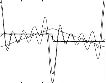
Fig. 6.8.1. Pressure (heavy solid) and R-scaled total flow wave (tot) through the RLC system in parallel, with the inertial time constant tL = 0.1 s and the capacitive time constant tC = 0.01 s. The dashed curves show the resistive (res), inductive (ind), and capacitive (cap) flows. It is seen that with these values of the time constants, flow through the system is dominated by the inductive and resistive components, capacitive flow is small by comparison. To facilitate the comparison, only the oscillatory parts of the pressure and flow waves are shown.

(mmHg)	1		tot
	0.5
flow
				res
R−scaled
	0
				cap
pressure,	−0.5
			ind
	−1
	0	0.2	0.4	0.6	0.8	1
			time t (normalized)

Fig. 6.8.2. See caption for Fig. 6.8.1.

216 6 Composite Pressure-Flow Relations

	15
(mmHg)	10		res
	5
flow
	0
R−scaled
				cap
	−5
	−10		ind
pressure,
	−15
	−20	tot
	−25
	0	0.2	0.4	0.6	0.8	1
			time t (normalized)

Fig. 6.8.3. See caption for Fig. 6.8.1.

The relation between the pressure and flow harmonics for the individual parallel flows is the same as that for the harmonics of total flow, that is, as in Eq. 6.8.7, here

Mnei(ωn t−φn )

qnr,res(t) = (6.8.16)

Zn,res

Mnei(ωn t−φn )

qnr,ind(t) = (6.8.17)

Zn,ind

Mnei(ωn t−φn )

qnr,cap(t) = (6.8.18)

Zn,cap

Evaluating these by following the step as before, and omitting the details, we find

R × qnr,res(t) = Mn cos (ωnt − φn)					(6.8.19)
R × qnr,ind(t) =		n	ωntL −		(6.8.20)
	M		sin (ωnt	φn)
R × qnr,cap(t) = −ωntC Mn sin (ωnt − φn)					(6.8.21)

The individual parallel flow waves shown in Figs. 7.3.1–3 are obtained by adding the harmonics of each flow, that is,

R × qr,res(t) = R × q1r,res + R × q2r,res + . . . + R × qN r,res (6.8.22)

6.8 Composite Pressure-Flow Relations Under RLC in Parallel

217

R × qr,ind(t) = R × q1r,ind + R × q2r,ind + . . . + R × qN r,ind (6.8.23)

R × qr,cap(t) = R × q1r,cap + R × q2r,cap + . . . + R × qN r,cap (6.8.24)

Only the oscillatory parts of pressure and flow waves are shown, the steady parts are omitted to make the graphical comparison easier by using the same scale.

The results in Figs. 6.8.1–3 indicate that with tL = 0.1 s and tC = 0.01 s capacitance e ects are small and total flow is dominated by inertial e ects. By contrast, when inductance and capacitance are in series, the same values of the time constants lead to a flow dominated by capacitive e ects as seen earlier in Figs. 6.7.1–3. If the capacitive time constant is increased to tC = 0.3 s, which means higher compliance (a more elastic balloon), keeping the inertial time constant unchanged, total flow becomes dominated by capacitive e ects as seen in Figs. 6.8.4–6. Because the two elements are in parallel, however, this does not change the resistive and the inductive flows.

(mmHg)	4
	2		tot
				ind
flow
R−scaled	0
			cap	res
	−2
pressure,
	−4
	−60	0.2	0.4	0.6	0.8	1
			time t (normalized)

Fig. 6.8.4. Pressure (heavy solid) and R-scaled total flow wave (tot) through the RLC system in parallel, as in Figs. 6.8.1–3, with the value of the inertial time constant unchanged at tL = 0.1 s but the value of the capacitive time constant is increased to tC = 0.3 s. The increase in the value of tC corresponds to higher compliance (a more elastic balloon), hence total flow is seen to be dominated by capacitive e ects. The resistive (res) and inductive (ind) flows are una ected by this change because the elements are in parallel.

218 6 Composite Pressure-Flow Relations

	1.5	cap		tot
(mmHg)	1
	0.5
flow	0	res
R−scaled	−0.5
	−1	ind
	−1.5
pressure,
	−2
	−2.5
	−3
	0	0.2	0.4	0.6	0.8	1
			time t (normalized)

Fig. 6.8.5. See caption for Fig. 6.8.4.

flow (mmHg)	60
			cap
	40
	20
R−scaled
	0		res
pressure,
	−20		ind
		tot
	−40
	0	0.2	0.4	0.6	0.8	1
			time t (normalized)

Fig. 6.8.6. See caption for Fig. 6.8.4.

6.9 Summary

219

6.9 Summary

Coronary blood flow may be disrupted by an obstruction in the vessels conveying the flow or by a disruption in the delicate dynamics of the flow, the dynamics of the coronary circulation. The focus in this book is on the latter. At the core of the dynamics of the coronary circulation is the relation between the form of the composite pressure wave driving the flow and the form of the resulting flow wave.

The simple relation between the amplitudes and phase angles of pressure and flow sine and cosine waves cannot be applied when pressure and flow are composite waves, but they can be applied to their individual harmonics. Furthermore, the flow contributions from individual harmonics can then be added to obtain the composite flow wave because the equation governing the flow is linear.

When the opposition to flow consists of pure resistance, a composite pressure wave produces a composite flow wave of identical form but shifted by only the units of pressure and flow. For the study of pressure-flow relations it is convenient to remove this shift so that the two waves actually coincide. This can be done by scaling the flow wave by the resistance. The resulting “R-scaled” flow wave is useful not only when the resistance to flow consists of pure resistance but also, and particularly, when inertial and capacitive e ects are involved too.

The flow wave associated with a composite pressure wave cannot be obtained directly and in full when opposition to flow consists of general impedance rather than pure resistance. In this case, direct pressure-flow relations exist only between the individual harmonics of pressure and flow. Thus, harmonics of the flow wave must be obtained individually first, then these are used to construct the flow wave as a whole.

Inertial e ects can lead to large swings in the R-scaled flow waveform, away from the corresponding pressure waveform. When the inductor is in series with a resistor, as is the case in the physiological system under normal circumstances, these swings are controlled by the presence of the resistor. When the two elements are in parallel, however, flow swings may be very large as they are free from the e ects of the resistor. While in the coronary circulation a parallel inductive flow can only occur in the presence of a breach within the coronary vasculature, the results indicate clearly that any change in e ective inductance L, locally or of the system as a whole, may upset the delicate dynamics of the system and hence the relation between pressure and flow. Drugs a ecting the consistency of blood or the caliber of blood vessels, for example, which are generally considered as targeting only the resistance to flow, will actually also alter inertial e ects within the system.

Like inertial e ects, capacitive e ects can lead to large swings in the R- scaled flow waveform, away from the corresponding pressure waveform. When the capacitance is in series with the resistance, these swings are constrained by the presence of the resistance, but when the two elements are in parallel,