The Physics of Coronory Blood Flow - M. Zamir

230 7 Lumped Models

Z =	1	(purely elastic capacitance)	(7.3.3)
	iωC

Following the same step as in Section 4.9 to find the complex impedance for a viscoelastic capacitor, we consider an oscillatory pressure in complex exponential form

p(t) = p0eiωt

(7.3.4)

where p0 is a constant, and substitute in Eq. 7.3.2 to get

B	dq	+		1	q = ip0ωeiωt	(7.3.5)
	dt
			C

To find the complex impedance we solve this equation for q(t), recalling from Section 4.9 that only the particular part of the solution is required. Following the same steps as in Section 4.9, we readily find

ip0ωeiωt q(t) = iBω + C1

Using Eq. 7.3.4 for p(t) and rearranging, this becomes

p(t) q(t) = B + iωC1

or

q(t) = p(t)

Z

where

1

Z = B + iωC

(7.3.6)

(7.3.7)

(7.3.8)

(7.3.9)

Comparing this with the results in Section 4.9, we see that the complex impedance for viscoelastic capacitance is the same as that for a purely elastic capacitance plus a resistance in series, as in Eq. 6.6.1, namely

Z = R +	1	(viscoelastic capacitance)	(7.3.10)
	iωC

Thus, to incorporate viscoelasticity into the windkessel model we simply add a resistance in series with the purely elastic capacitance in that model, which leads to the model shown in Fig. 7.3.1. In current notation the resulting model is {R1 + {R2 + C}} and we shall refer to it as LM 1. It is sometimes referred to as the viscoelastic windkessel model.

The two resistances R1, R2 in this model are clearly di erent and for modelling purposes must be allowed to assume di erent values. We shall find that if we continue to use the concept of R-scaled flow as being the product of

7.3 LM1: {R1,{R2+C}} 231

LM1

qtot

R1	R2
qres	qcap
	C

Fig. 7.3.1. A modified (viscoelastic) “windkessel” model in which capacitance is assumed to be not purely elastic as in LM 0 but viscoelastic, which is equivalent to having a purely elastic capacitance C in series with a resistance R2. Total flow through the system then consists of qres along one of the two parallel branches and qcap along the other.

resistance and flow, namely R × q, and if we now use R1 in this product, that is define R-scaled flow as R1 × q, then only the ratio of the two resistances is required subsequently. In other words, if we introduce

	λ =	R2	(7.3.11)
		R1

then only the value of λ is required in subsequent analysis.

The complex impedances along the two branches of LM 1, using results in Section 4.9, are given by

Zres = R1		(7.3.12)
1
Zcap = R2 +		(7.3.13)
	iωC

For convenience, we continue to refer to the two branches of the model as the “resistive” branch and the “capacitive” branch even though there is resistance in both branches. The complex impedance for the entire system is then given by

232 7 Lumped Models

	1	=	1	+	1		(7.3.14)
	Z		Zres		Zcap
	Z =		R1	+ iωR1R2C			(7.3.15)
			1 + iωC(R1 + R2)

where ω is the angular frequency of oscillation of the driving pressure. For the individual harmonics of a composite pressure wave consisting of N harmonics, in the notation of the previous section, we then have

Zn,res = R1				(7.3.16)
1				(7.3.17)
Zn,cap = R2 +
		iωnC
Zn =	R1 + iωnR1R2C			(7.3.18)
	1 + iωnC(R1 + R2)

where n denotes a particular harmonic and ωn is the angular frequency of that harmonic.

For a composite pressure wave consisting of the following harmonics (in their complex exponential form)

pn(t) = Mnei(ωn t−φn ) n = 1, 2, . . . , N

(7.3.19)

we obtain the corresponding harmonics of the flow wave, as in Chapter 6,

qnr (t) =	pn(t)
	Zn
=		Mnei(ωn t−φn )
	(R1 + iωnR1R2C)/(iωnR1C)

=[(1 + ωn2 C2R2(R1 + R2))Mn cos (ωnt − φn)

−ωnR1CMn sin (ωnt − φn)]/[R1(1 + (ωnR2C)2)]

or in R-scaled form

R1 × qnr (t) = [(1 + ωn2 t2C λ(1 + λ))Mn cos (ωnt − φn) −ωntC Mn sin (ωnt − φn)]/[1 + (ωnλtC )2]

(7.3.20)

(7.3.21)

(7.3.22)

(7.3.23)

where tC is the capacitive time constant (= R1C). Similarly, and omitting the details, we find the R-scaled resistive and capacitive flows

pn(t)

qnr,res(t) = (7.3.24)

Zn,res

R1 × qnr,res(t) = Mn cos (ωnt − φn)

(7.3.25)

7.3 LM1: {R1,{R2+C}} 233

			qnr,cap(t) =				pn(t)	(7.3.26)
							Zn,cap
R	1	×	q	nr,cap	(t) = ωn2 tC2 λMn cos (ωnt − φn) − ωntC Mn sin (ωnt − φn)
								1 + (ωnλtC )2

(7.3.27)

Finally, the total and the two parallel flow waves are obtained by adding the harmonics of each flow, that is, in R-scaled format

R1 × qr (t) = R1 × q1r (t) + R1 × q2r (t) . . . + R1 × qN r (t) (7.3.28)

R1 × qr,res(t) = R1 × q1r,res + R1 × q2r,res + . . . + R1 × qN r,res (7.3.29)

R1 × qr,cap(t) = R1 × q1r,cap + R1 × q2r,cap + . . . + R1 × qN r,cap (7.3.30)

As before, only the oscillatory parts of the pressure and flow waves are used, the steady parts being omitted to make the graphical comparison of these waves easier by using the same scale.

Results, demonstrating the e ects of viscoelasticity on the relation between pressure and flow waves are shown in Figs.7.3.2-4. In all three figures the value

	40					LM1
(mmHg)
	30
	20
flow			tot
R−scaled	10
	0		cap	p, res
pressure,	−10
	−20
	−30
	0	0.2	0.4	0.6	0.8	1
			time t (normalized)

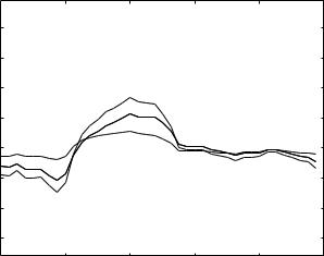
Fig. 7.3.2. Pressure-flow relations under LM 1 with the same value of the capacitive time constant as in Fig. 7.2.3 of the purely elastic windkessel model, namely tC = 0.2 s, but here with the addition of viscoelastic e ects in the vessel wall. A measure of these e ects is the value of the parameter λ = R2/R1 where R2 is a resistance in series with a purely elastic capacitance and R1 is a resistance in parallel with it. Results in this figure are based on λ = 2.0, which seems su cient to produce dramatic change in the forms of the R-scaled capacitive (cap) and total (tot) flow waves compared with those in Fig. 7.2.3. The heavy solid curve represents the pressure wave (p) as well as the R-scaled resistive flow wave (res).

234 7 Lumped Models

	40					LM1
(mmHg)
	30
	20
flow			tot
R−scaled	10
	0		cap	p, res
pressure,	−10
	−20
	−30
	0	0.2	0.4	0.6	0.8	1
			time t (normalized)

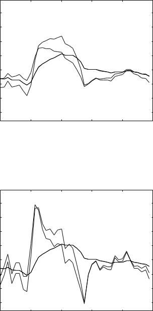
Fig. 7.3.3. Pressure-flow relations under LM 1 as in Fig. 7.3.2 but here with reduced viscoelastic e ect, namely λ = R2/R1 = 0.5.

	40					LM1
(mmHg)
	30
	20
flow			tot
R−scaled	10			p, res
	0		cap
pressure,	−10
	−20
	−30
	0	0.2	0.4	0.6	0.8	1
			time t (normalized)

Fig. 7.3.4. Flow under LM 1 but with considerably reduced viscoelastic e ect, namely λ = R2/R1 = 0.1. Viscoelastic e ects at this value of λ are practically insignificant, and the total flow wave is again dominated by an erratic form of the capacitive flow as in Fig. 7.2.3 of the purely elastic windkessel model.

7.4 LM2: {{R1+L},{R2+C}} 235

of the capacitive time constant is taken to be the same as that in Fig. 7.2.3 of the purely elastic windkessel model in the previous section, namely tC = 0.2 s. In addition to this, the value of λ (= R2/R1) is required in the present model as a measure of the degree of viscoelasticity. In Fig. 7.3.2, results are shown with λ = 2.0. Comparison of these results with those in Fig. 7.2.3 show dramatically the e ects of viscoelasticity on the form of the flow wave. Chaotic wave swings are entirely eliminated, and the flow wave follows the form of the pressure wave rather than the form of its slope as in Fig. 7.2.5. This dramatic e ect diminishes as the value of λ is reduced, as shown in Figs. 7.3.3, 4. A reduction in the value of λ corresponds to a reduction in the value of R2 relative to that of R1, which in turn corresponds to a reduction in the viscoelastic property of the vessel wall.

7.4 LM2: {{R1+L},{R2+C}}

The modified windkessel model of the previous section lacks an important element of the RLC system, namely the inductor L which represents inertial e ects as discussed in Section 2.5. With a few exceptions [203, 188, 75], inductance has not usually been included in lumped models of the coronary circulation, possibly because inertial e ects are usually associated with the transient dynamics of the system rather than the steady state dynamics which lumped models deal with. It must be remembered, however, that even within steady state dynamics, within the oscillatory cycle, fluid is being accelerated and decelerated and therefore inertial e ects will play a role. It is a di erent role from that which inertial e ects play in the transient state, where the effects are represented by exponential functions that die out as time goes on. In steady state, inertial e ects have a permanent cyclic presence which does not die out and which, as we shall see, a ects the dynamics of the system and the relation between pressure and flow waveforms.

The position of an inductor in a lumped model of the coronary circulation is fairly clear because acceleration and deceleration of the flow within the oscillatory cycle occur along the conducting vessels rather than within the capacitor. Acceleration and deceleration associated with capacitance is usually minimal because it involves mainly local inflation and deflation of the vessels. Flow along the vessels, on the other hand, involves considerable acceleration and deceleration and hence considerable inertial e ects. And these inertial e ects are coupled with the viscous resistance within the conducting vessels such that the flow is subject to both, without an “either/or” option. By contrast, the capacitance e ects and the viscous resistance are “either/or” options because the flow may inflate the vessels or move along them. Thus, the capacitance C in a lumped model of the coronary circulation is appropriately placed in parallel with the viscous resistance R1, as in LM 0 and LM 1. Inductance L, on the other hand, is appropriately placed in series with that resistance as shown in Fig. 7.4.1, which we shall refer to as LM 2.

236 7 Lumped Models

LM2

qtot

R1

R2

L	qcap
	C

qind

Fig. 7.4.1. A viscoelastic lumped model with an inductor (L) representing inertial e ects of fluid acceleration and deceleration within the oscillatory cycle. Total flow into the system (qtot) consists of two parallel flows: inductive flow (qind) and capacitive flow (qcap). The inductor L is in series with a resistor R1 representing the viscous resistance along the conducting vessels, while the capacitor C is in series with a resistor R2 representing viscoelasticity within the vessel wall.

The complex impedances along the two parallel branches of LM 2, which we shall refer to as the capacitive (cap) and inductive (ind) branches, are obtained from the results of Section 4.9, namely

Zind = R1	+ iωL		(7.4.1)
	1		(7.4.2)
Zcap = R2	+
		iωC

and the complex impedance for the entire system is then given by

	1	=	1	+		1			(7.4.3)
					Zcap
	Z		Zind
	Z =		(R1 + iωL)(1 + iωR2C)						(7.4.4)
			1 + iωC(R2 + R1 + iωL)

where ω is angular frequency of the oscillatory driving pressure. For the individual harmonics of a composite pressure wave consisting of N harmonics, in

7.4 LM2: {{R1+L},{R2+C}}

the notation of the previous section, we then have

Zn,ind = R1 + iωnL

1

Zn,cap = R2 + iωnC

	Zn =	(R1 + iωnL)(1 + iωnR2C)
		1 + iωnC(R2 + R1 + iωnL))

237

(7.4.5)

(7.4.6)

(7.4.7)

where n denotes a particular harmonic and ωn is the angular frequency of that harmonic.

For a composite pressure wave consisting of the following harmonics (in their complex exponential form)

pn(t) = Mnei(ωn t−φn ) n = 1, 2, . . . , N

(7.4.8)

we obtain the corresponding harmonics of the R-scaled flow waves, as in Chapter 6, but omitting a considerable amount of algebra

			qnr,ind		(t) = Zn,ind
							pn(t)
R	1	×	q	nr,ind	(t) =	Mn cos (ωnt − φn) + ωntLMn sin (ωnt − φn)
							1 + ωn2 tL2

pn(t)

qnr,cap(t) =

Zn,cap

(7.4.9)

(7.4.10)

(7.4.11)

R

1

×

q

nr,cap

(t) =

ωn2 tC2 λMn cos (ωnt − φn) − ωntC Mn sin (ωnt − φn)

(7.4.12)

1 + ωn2 tC2 λ2

qnr (t) =

pn(t)

(7.4.13)

Zn

R

1

×

q

nr

(t) = [1 + ωn2 tC2 λ]{Mn cos (ωnt − φn) + ωntLMn sin (ωnt − φn)}

(1 + ωn2 tL2 )(1 + (ωn2 tC2 λ2)

+ [1 + ωn2 tL2 ]{ωn2 tC2 λMn cos (ωnt − φn) − ωntC Mn sin (ωnt − φn)}

(1 + ω2 t2 )(1 + ω2 t2 λ2)

n L

n C

(7.4.14)

where, as before (Eq. 7.3.11), λ = R2/R1. Finally, the total and the two parallel flow waves are obtained by adding the harmonics of each flow, that is, in R-scaled format

238 7 Lumped Models

R1 × qr (t) = R1	× q1r (t) + R1 × q2r (t) . . . + R1 × qN r (t) (7.4.15)
R1 × qr,ind(t) = R1	× q1r,ind + R1 × q2r,ind + . . . + R1 × qN r,ind (7.4.16)
R1 × qr,cap(t) = R1	× q1r,cap + R1 × q2r,cap + . . . + R1 × qN r,cap (7.4.17)

As before, only the oscillatory parts of the pressure and flow waves are used, the steady parts being omitted to make the graphical comparison of these waves easier by using the same scale.

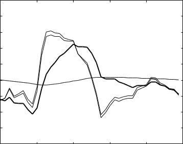
Results based on this model require that three parameters be specified, namely the capacitive and inertial time constants tC , tL, and the ratio λ (= R2/R1). To examine particularly the role of inertial e ects, results for a relatively high value of tL are compared with results for a relatively low value in Figs. 7.4.2, 3. It is seen that at a high value of tL flow along the inductive branch of the system is considerably reduced, with the result that total flow into the system is dominated by flow along its capacitive branch. At the other extreme, where tL is low, flow along the inductive branch is fairly high to the extent that total flow into the system is now closer in form to that of the pressure wave rather than that of the capacitive wave.

	25
	20					LM2
(mmHg)
	15		cap
			tot
	10
flow				p
	5
R−scaled
	0		ind
	−5
pressure,
	−10
	−15
	−200	0.2	0.4	0.6	0.8	1
			time t (normalized)

Fig. 7.4.2. Flow waves under LM 2 and a composite driving pressure wave (p), with tC = 0.2 s, λ = 0.5, and a relatively high value of the inertial time constant, namely tL = 1.0 s. Flow along the inductive branch (ind) of the system is small and total flow (tot) is dominated by flow along the capacitive branch (cap) of the system.

				7.4 LM2: {{R1+L},{R2+C}}		239
	25
	20				LM2
(mmHg)
	15		tot
		cap
	10
flow
	5		p
R−scaled
	0		ind
	−5
pressure,
	−10
	−15
	−200	0.2	0.4	0.6	0.8	1
			time t (normalized)

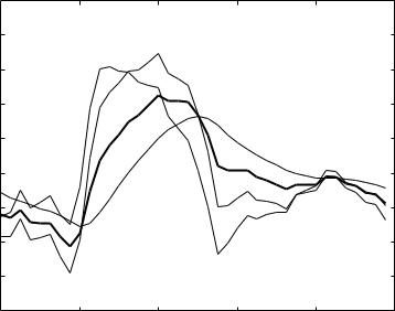
Fig. 7.4.3. Flow waves under LM 2 and a composite driving pressure wave (p), as in Fig. 7.4.2 but with a relatively low value of the inertial time constant, namely tL = 0.1 s. Inductive (ind) and capacitive (cap) flows are both high, but their forms are complimentary, their highs and lows nearly balancing each other, leaving total flow (tot) closer in form to that of the composite pressure wave (p).

The results in Fig. 7.4.3 in fact suggest the possibility that the most important role which inertial e ects may play in the dynamics of the coronary circulation is that of acting as a balance for capacitive e ects. Thus, with the combination of parameter values in Fig. 7.4.3 it is seen that the highs and lows of the capacitive and inductive flows almost balance each other, suggesting that a combination of parameters may exist at which the two flows exactly balance each other. Indeed, a close scrutiny of Eq. 7.4.14 shows that when

λ = 1.0 and tL = tC

(7.4.18)

the equation reduces to

R1 × qnr (t) = Mn cos (ωnt − φn)	(7.4.19)
= Mnei(ωn t−φn )	(7.4.20)

which means that the R-scaled total flow wave has become identical in form to that of the driving pressure. Under these conditions it is as if the inductor