The Physics of Coronory Blood Flow - M. Zamir

5.4 Example: Piecewise Waveform

159

= 2

0

1 p(t) cos (2nπt)dt

(5.4.14)

0

1/4

1/2

= 2

4t cos (2nπt)dt + 2

1/4

cos (2nπt)dt

3/4 1

1

+2

1/2

cos (2nπt)dt +

3/4

0 × dt

(5.4.15)

2

cos (2nπt)

(2nπt)

1/4

= 4

+

t sin

0

2(nπ)2

nπ

sin (2nπt)

1/2

sin (2nπt)

3/4

1/4

+

nπ

+

2nπ

1/2

+ 0

(5.4.16)

2

nπ

1

3nπ

=

cos

− 1 +

sin

(5.4.17)

(nπ)2

2

2nπ

2

where the first integral in Eq. 5.4.15 was evaluated using integration by parts, with the standard result [80, 186, 25]

cos kx

x sin kx

(5.4.18)

x cos kxdx =

+

k2

k

2

T

2nπt

Bn =

0

p(t) sin

dt

(5.4.19)

T

T

=

2

0

1 p(t) sin (2nπt)dt

(5.4.20)

0

1/4

1/2

=

2

4t sin (2nπt)dt + 2

1/4

sin (2nπt)dt

3/4 1

1

+2

1/2

sin (2nπt)dt + 3/4

0 × dt

(5.4.21)

2

=

4

2(nπ)2

− t cosnπ

1/4

0

sin (2nπt)

(2nπt)

3/4

1/2

cos (2nπt)

cos (2nπt)

−

nπ

1/4

−

2nπ

1/2

+ 0

(5.4.22)

2

nπ

1

−

1

3nπ

(nπ)2

2

− 2nπ

2nπ

2

=

sin

cos (nπ)

cos

(5.4.23)

Here, again, the first integral in Eq. 5.4.21 was evaluated using integration by parts, with the standard result [80, 186, 25]

	x sin kxdx =	sin kx		−	x cos kx		(5.4.24)
		k2			k

160 5 The Analysis of Composite Waveforms

Substitution of these expressions for the Fourier coe cients in Eqs.5.4.6 makes the resulting expression for the Fourier series rather cumbersome. Instead, numerical values of An, Bn, Mn, φn can be simply tabulated for the required number of harmonics, as shown in Table 5.4.1.

Table 5.4.1. Numerical values of Fourier coe cients for the first ten harmonics of the piecewise waveform shown in Fig. 5.4.1.

n	An	Bn	Mn	φn (deg)
1	-0.36180	0.36180	0.51166	135
2	-0.10132	0.00000	0.10132	180
3	0.03054	0.03054	0.04318	45
4	0.00000	-0.07958 0.07958		-90
5	-0.03994	0.03994	0.05648	135
6	-0.01126	0.00000	0.01126	180
7	0.01860	0.01860	0.02631	45
8	0.00000	-0.03979 0.03979		-90
9	-0.02019	0.02019 0.02855		135
10	-0.004053	0.00000 0.00405		180

Values of Mn in Table 5.4.1 are determined as before, namely from

(Eq. 5.3.24)
Mn = An2 + Bn2	(5.4.25)

However, as mentioned in the previous section, the phase angles φn must satisfy both conditions in Eqs.5.2.23,24, namely

An = Mn cos φn				(5.4.26)
Bn = Mn sin φn				(5.4.27)
These two conditions cannot be replaced by the single condition
	Bn
φn = tan−1				(5.4.28)
		An

because the range of values of the inverse tangent function is limited to the interval −π/2 to π/2. For example, using the values of A1, B1 from the table, Eq. 5.4.28 gives

				B1
φ1 = tan−1							(5.4.29)
				A1
			0.3618
= tan−1							(5.4.30)
				−0.3618
= tan−1(−1)							(5.4.31)
= −	π						(5.4.32)
	4

5.4 Example: Piecewise Waveform

161

This value of φ1 is incorrect because it does not satisfy Eqs.5.4.26,27. Substituting φ1 = −π/4 in these equations gives

A1 =	M1 cos (−π/4)	(5.4.33)
=	0.51166 × 0.7071	(5.4.34)
=	0.3618	(5.4.35)
B1 = M1 sin (−π/4)		(5.4.36)
= 0.51166 × (−0.7071)		(5.4.37)
= −0.3618		(5.4.38)

imaginary axis

(A,B)

φ

real axis

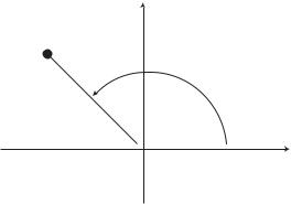
Fig. 5.4.2. The phase angle φ of a harmonic with coe cients A, B is correctly obtained as the argument of the complex number z = A + iB. This angle, φ = arg(z), is measured in an anticlockwise direction from the real axis, as shown, and has the range of values −π to π. The example shown here is that of the first harmonic of the piecewise waveform for which the values of the coe cients (from Table 5.4.1) are A1 = −0.3618 and B1 = 0.3618, which are shown in the complex plane above as the coordinates of the complex number z, and which give φ = arg (−0.3618 + i × 0.3618) = 3π/4 = 135◦ as given in Table 5.4.1. The in-

verse tangent function in this case would give an incorrect value, namely φ = tan−1(B/A) = tan−1(−1) = π/4 = 45◦ .

These values of A1, B1 are incorrect, the actual values are A1 = −0.3618, B1 = 0.3618 as indicated in the table. The correct value of φ1, that is, a value of φ1 which satisfies both of Eqs.5.4.26,27, is actually 3π/4 or 135◦ as indicated in the table. This value is obtained by writing A1, B1 as the real and imaginary parts of a complex number

z1 = A1 + iB1

(5.4.39)

162 5 The Analysis of Composite Waveforms

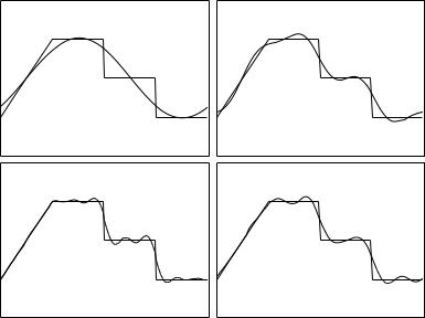
Fig. 5.4.3. Fourier series representations of the piecewise waveform in Fig. 5.4.1, based on the first one, four, seven, and ten harmonics, clockwise from top left corner.

then the correct value of φ1 is obtained as the argument (“arg”) of z1, that is

φ1 = arg(z1)

(5.4.40)

where the function “arg” is the angle of a complex number in the complex plane or Argand diagram, measured in an anticlockwise direction from the real axis and having the range of values −π to π, as illustrated in Fig. 5.4.2.

Numerical values of the coe cients A1, B1 can now be extracted from Table 5.4.1 to construct the Fourier series representation of the piecewise waveform in its full form, as in Eq. 5.2.14, giving

∞

2nπt

∞

nπt

(5.4.41)

p(t) = n=0 An cos

T

+ n=1 Bn sin

2 T

= A0 + A1 cos

2T

+ A2 cos

T

+ ...

πt

4πt

πt

4πt

+B1 sin

2

+ B2 sin

+ ...

(5.4.42)

T

T

=0.5 − 0.3618 × cos (2πt) − 0.10132 × cos (4πt) +0.030536 × cos (6πt) + 0.3618 × sin (2πt)

+0.030536 × sin (6πt) + ...

(5.4.43)

Or, numerical values of Mn, φn can be used from Table 5.4.1 to put the series in its compact form, as in Eqs.5.2.21,22

5.4 Example: Piecewise Waveform

163

	1.5
	1
magnitude	0.5
	0
	−0.50	0.2	0.4	0.6	0.8	1
				time

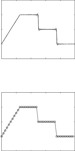
Fig. 5.4.4. Fourier series representation of the piecewise waveform in Fig. 5.4.1, based on the first 50 harmonics.

magnitude

1.5

1

0.5

0
−0.50	0.2	0.4	0.6	0.8	1
			time

Fig. 5.4.5. Fourier series representation (circles) of the piecewise waveform in Fig. 5.4.1 (solid line) based on a Fast Fourier Transform (FFT) algorithm.

164 5 The Analysis of Composite Waveforms
p(t) = A0	+ n=0 Mn cos			2 T	− φn			(5.4.44)
	∞			nπt
			2T		+ M2 cos	T
= A0	+ M1 cos			− φ1			− φ2
			πt			4πt

+M3 cos	6πt	− φ3	+ ...	(5.4.45)
	T

=0.5 + 0.51166 × cos (2πt − 135 × π/180) +0.10132 × cos (4πt − 180 × π/180)

+0.043184 × cos (6πt − 45 × π/180) + ...

(5.4.46)

As in the previous example, if the harmonics of this waveform are denoted by p1(t), p2(t), p3(t) etc., then the individual harmonics are given by

p1	(t) = 0.51166 × cos (2πt − 135 × π/180)	(5.4.47)
p2	(t) = 0.10132 × cos (4πt − 180 × π/180)	(5.4.48)
p3	(t) = 0.043184 × cos (6πt − 45 × π/180)	(5.4.49)
	.
	.
	.
p10	(t) = 0.0040528 × cos (20πt − 180 × π/180)	(5.4.50)

Again, it is seen that the first harmonic has the same period and hence the same frequency as the original wave, namely the fundamental period and fundamental frequency. The period of the second harmonic is one half of the fundamental period and hence its frequency is twice the fundamental frequency, etc. The first ten harmonics are shown graphically in Fig. 5.4.1.

Fig. 5.4.3 shows the accuracy of this Fourier representation of the piecewise waveform when only the first one, four, seven, and ten harmonics are used. A Fourier representation with the first 50 harmonics is shown in Fig. 5.4.4, and a representation based on a computer based Fast Fourier Transform is shown in Fig. 5.4.5.

5.5 Numerical Formulation

The waveforms considered in the previous two sections were rather artificially constructed in order to illustrate the basic concepts of Fourier analysis and the basic steps involved in its application to a specific waveform. In the context of the coronary circulation, however, the specific waveforms of interest are the pressure and flow waveforms generated by the pumping action of the left ventricle, as in the example shown in Fig. 5.1.2. One important feature of this waveform which is not shared by the examples of the previous two sections is that it cannot be presented in analytical form, as in Eqs.5.3.1,2 for the single-step waveform, or in Eqs.5.4.1-4 for the piecewise waveform.

5.5 Numerical Formulation

165

As stated in the introduction to this chapter, a cardiac pressure waveform of the type shown in Fig. 5.1.2 is generally available only in numerical form, that is as a set of points, tabulated as in Table 5.1.1 or presented graphically as in Fig. 5.1.2. This is the most natural way in which the waveform would present itself in practice where the set of points would come from pressure or flow measurements at some accessible point within the coronary vasculature, at small time intervals during the oscillatory cycle as shown in Table 5.1.1.

The aim of the present section is to show how such a set of points would be used in the process of Fourier analysis to produce the Fourier series representation of the waveform. Once this representation has been achieved, the waveform becomes like any other waveform, expressed in terms of a series of sine and cosine functions, or in terms of its harmonics as in the examples of the previous sections. Indeed, the data in Table 5.1.1 may be regarded as a periodic function like any other we have considered so far, the only di erence here is that the function is presented in numerical form rather than analytically. Each pair of values (p, t) in the table represents one point in Fig. 5.1.2, and the entire set of values in the table produce the waveform shown in the figure.

Let the number of points available be denoted by N , which is not to be confused with n which we shall continue to use for the number of harmonics. The Fourier analysis process is considerably easier, of course, when the points are spaced at regular intervals of time within the oscillatory cycle, and we shall proceed on that assumption. In fact, if the original set points are not equally spaced in time, it would be best first to place them on a “best-fit” curve and then extract a new set of points from that curve at regular time intervals. It is also easier, particularly when using Fast Fourier Transform (FFT) programs, if N is an even number.

If the period of the waveform is denoted by T , and the time interval be-

	tween successive data points is denoted by Δt, then
	Δt =	T		(5.5.1)
		N

In Table 5.1.1 the period has been normalized to T = 1.0 and the number of points N = 40, therefore Δt = 1/40 = 0.025 as noted from successive points in the table.

If the time at the beginning of the oscillatory cycle is set at t = 0, and if this and subsequent points in time are denoted by t0, t1, t3 etc., then these points are given by

t0 = 0

t1 = 1 × Δt t2 = 2 × Δt t3 = 3 × Δt

.

.

.

166 5 The Analysis of Composite Waveforms

tN −1 = (N − 1) × Δt

(5.5.2)

Note that there are a total of N points in time within one oscillatory cycle. If the corresponding values of p(t) are denoted similarly by p0, p1, p2 etc., then

p0	= p(t0)
p1	= p(t1)
p2	= p(t2)
p3	= p(t3)
	.
	.
	.
pN −1	= p(tN −1)	(5.5.3)

The general form of the Fourier series representation of the cardiac waveform in Fig. 5.1.2 is the same as for other waveforms, namely

∞

nπt

∞

2nπt

(5.5.4)

p(t) = n=0 An cos

2 T

+ n=1 Bn sin

T

4T

= A0 + A1 cos T

+ A2 cos

+ ...

2πt

πt

2T

+B1 sin

+ B2 sin T

+ ...

(5.5.5)

πt

4πt

but the Fourier coe cients An, Bn in the present case cannot be evaluated by means of integrals as before, because the periodic function p(t) is not available in analytical form. But the function is available in numerical form, as in Table 5.1.1, therefore the required integrals can be formulated and evaluated numerically in a fairly straightforward manner as shown below.

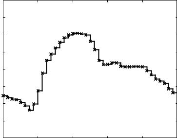
If each of the N points describing the periodic function p(t) is associated with one time interval Δt, then the N points together cover the entire period T . In the simplest numerical formulation, the value of the function p(t) at t0, namely p0, is taken to remain constant over the small time interval Δt associated with t0, then the value of p(t) at t1, namely p1, is taken to remain constant over the next time interval, etc., with the result that the periodic function p(t) is presented graphically as shown in Fig. 5.5.1. This graphical presentation provides the basis for the numerical formulation and evaluation of the Fourier coe cients An, Bn.

Briefly, each of the integrals required in the evaluation of the coe cients is reformulated as a sum, using standard methods. Thus, for A0 we have (Eq. 5.2.15)

		1	0	T
	A0 =			p(t)dt	(5.5.6)
		T

5.5 Numerical Formulation

167

	20
	15
	10
(p)	5
magnitude	0
	−5
	−10
	−15
	−200	0.2	0.4	0.6	0.8	1

time (t)

Fig. 5.5.1. Graphical presentation of the periodic function p(t), when the description of the function is available only numerically. The data points shown are based on the data in Table 5.1.1 for the cardiac waveform in Fig. 5.1.1. In a numerical formulation of Fourier analysis, each data point is associated with the small time interval Δt between it and the next data point, and over each such Δt the value of p is taken to remain constant as shown in the figure. This allows the numerical formulation and evaluation of the Fourier coe cients An, Bn as described in the text.

The integral on the right in fact represents the area under the curve representing the function p(t) over one period. The graphical presentation in Fig. 5.5.1 shows that to a good approximation this area is equal to the sum of the areas of the N long thin rectangles of width Δt rising from the t axis to the curve. This makes it possible to write

A0 =		1		{p0Δt + p1Δt + p2Δt . . . pN −1Δt}	(5.5.7)
	T
=		1		{p0 + p1 + p2 + . . . + pN −1} Δt	(5.5.8)
	N
		Δt N −1
=					(5.5.9)
				pk
		N		k=0

having used Eq. 5.5.1 in the process.

168 5 The Analysis of Composite Waveforms

Numerical expressions for An and Bn are obtained in the same way, although the integrals in this case involve the product of p(t) and a sine or cosine function and therefore do not represent simply the area under the p(t) curve. Nevertheless, using the integral expressions for these coe cients from Eqs.5.2.16,17 and converting the integrals involved into sums as for A0, we find

An = T

T

T

dt

0

p(t) cos

2

2nπt

= T

p0 cos

T

0

Δt + p1 cos

T

1

Δt + . . .

2

2nπt

2nπt

2nπtN −1

+ pN −1 cos

T

T

Δt

T

+ . . .

= N

p0 cos

0

+ p1 cos

1

2

2nπt

2nπt

2nπtN −1

+ pN −1 cos

T

Δt

Δt N −1

2nπt

k

= 2N

k=0 pk cos

T

Bn = T

0

T

T

dt

p(t) sin

2

2nπt

p0 sin

Δt + . . .

= T

T

0

Δt + p1 sin

T

1

2

2nπt

2nπt

+ pN −1 sin

2nπtN −1

Δt

T

T

T

+ . . .

= N

p0 sin

0

+ p1 sin

1

2

2nπt

2nπt

+ pN −1 sin

2nπtN −1

Δt

T

Δt N −1

2nπt

k

= 2N

k=0 pk sin

T

(5.5.10)

(5.5.11)

(5.5.12)

(5.5.13)

(5.5.14)

(5.5.15)

(5.5.16)

(5.5.17)

These expressions are valid generally for any periodic function p(t) for which a numerical description is available in terms of N data points as in Table 5.1.1. The expressions are used specifically for that case in the next section.