Fitts D.D. - Principles of Quantum Mechanics[c] As Applied to Chemistry and Chemical Physics (1999)(en)

12 The wave function

Thus, the product of these two uncertainties Äx and Äk is a constant of order unity, independent of the parameter á.

Square pulse wave number distribution

As a second example, we choose A(k) to have a constant value of unity for k between k1 and k2 and to vanish elsewhere, so that

A(k) 1,	k1 < k < k2	(1:21)
0,	k , k1, k . k2

as illustrated in Figure 1.6(a). With this choice for A(k), the modulating function B(x, t) in equation (1.17) becomes

1

k2

…k1 ei(xÿvg t)(kÿk0) dk

B(x, t) p2ð

••••••

1

i(x

ÿ

vg t)(k2

ÿ

k0)

i(x

ÿ

vg t)(k1

ÿ

k0)

p2ði(x

t)

[e

ÿ e

]

••••••

1

ÿ vg

i(x

t)

k

2

i(x

t)

k 2

p

ÿ vg

[e

ÿvg

Ä

=

ÿ eÿ ÿvg

Ä =

]

••••••

t)

2ði(x

r•••

ÿ vg

2

sin[(x ÿ vg t)Äk=2]

(1:22)

ð

x

t

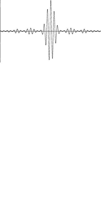
where k0 is chosen to be (k1 k2)=2, Äk is de®ned as (k2 ÿ k1), and equation (A.33) has been used. The function B(x, t) is shown in Figure 1.6(b).

The real part of the wave packet Ø(x, t) obtained from combining equations (1.14) and (1.22) is shown in Figure 1.7. The amplitude of the plane wave exp[i(k0 x ÿ ù0 t)] is modulated by the function B(x, t) of equation (1.22), which has a maximum when (x ÿ vg t) equals zero, i.e., when x vg t. The nodes of B(x, t) nearest to the maximum occur when (x ÿ vg t)Äk=2 equalsð, i.e., when x is (2ð=Äk) from the point of maximum amplitude. If we consider the half width of the wave packet between these two nodes as a measure of the uncertainty Äx in the location of the wave packet and the width (k2 ÿ k1) of the square pulse A(k) as a measure of the uncertainty Äk in the value of k, then the product of these two uncertainties is

ÄxÄk 2ð

Uncertainty relation

We have shown in the two examples above that the uncertainty Äx in the position of a wave packet is inversely related to the uncertainty Äk in the wave numbers of the constituent plane waves. This relationship is generally valid and

1.2 Wave packet

13

A(k)

1

(a)	0			k
		k1	k2

B(x, t)

Äk/√2ð

x 2 vg t

(b)

22ð/Äk 0

2ð/Äk

Figure 1.6 (a) A square pulse wave number distribution. (b) The modulating function corresponding to the wave number distribution in Figure 1.6(a).

Re Ø(x, t)

x

Figure 1.7 The real part of a wave packet for a square pulse wave number distribution.

14	The wave function

is a property of Fourier transforms. In order to localize a wave packet so that the uncertainty Äx is very small, it is necessary to employ a broad spectrum of plane waves in equations (1.11) or (1.17). The function A(k) must have a wide distribution of wave numbers, giving a large uncertainty Äk. If the distribution A(k) is very narrow, so that the uncertainty Äk is small, then the wave packet becomes broad and the uncertainty Äx is large.

Thus, for all wave packets the product of the two uncertainties has a lower bound of order unity

ÄxÄk > 1

(1:23)

The lower bound applies when the narrowest possible range Äk of values for k is used in the construction of the wave packet, so that the quadratic and higherorder terms in equation (1.13) can be neglected. If a broader range of k is allowed, then the product ÄxÄk can be made arbitrarily large, making the right-hand side of equation (1.23) a lower bound. The actual value of the lower bound depends on how the uncertainties are de®ned. Equation (1.23) is known as the uncertainty relation.

A similar uncertainty relation applies to the variables t and ù. To show this

relation, we write the wave packet (1.11) in the form of equation (B.21)
1		1	(1:24)
Ø(x, t) p2ð		…ÿ1G(ù)ei(kxÿùt) dù
••••••
where the weighting factor G(ù) has the form of equation (B.22)
1	1
G(ù) p2ð	…ÿ1Ø(x, t)eÿi(kxÿùt) dt
••••••

In the evaluation of the integral in equation (1.24), the wave number k is regarded as a function of the angular frequency ù, so that in place of (1.13) we have

k(ù) k0	dk	(ù ÿ ù0)
	dù 0

If we neglect the quadratic and higher-order terms in this expansion, then

equation (1.24) becomes			C(x, t)ei(k0 xÿù0 t)
Ø(x, t)
where
1	1
C(x, t) p2ð	…ÿ1 A(ù)eÿi[tÿ(dk=dù)0 x](ùÿù0) dù
••••••

As before, the wave packet is a plane wave of wave number k0 and angular frequency ù0 with its amplitude modulated by a factor that moves in the positive x-direction with group velocity vg, given by equation (1.16). Following

1.3 Dispersion of a wave packet

15

the previous analysis, if we select a speci®c form for the modulating function G(ù) such as a gaussian or a square pulse distribution, we can show that the product of the uncertainty Ät in the time variable and the uncertainty Äù in the angular frequency of the wave packet has a lower bound of order unity, i.e.

ÄtÄù > 1

(1:25)

This uncertainty relation is also a property of Fourier transforms and is valid for all wave packets.

1.3 Dispersion of a wave packet

In this section we investigate the change in contour of a wave packet as it propagates with time.

The general expression for a wave packet Ø(x, t) is given by equation (1.11). The weighting factor A(k) in (1.11) is the inverse Fourier transform of Ø(x, t) and is given by (1.12). Since the function A(k) is independent of time, we may set t equal to any arbitrary value in the integral on the right-hand side of equation (1.12). If we let t equal zero in (1.12), then that equation becomes

1	1	(1:26)
A(k) p2ð	…ÿ1Ø(î, 0)eÿikî dî
••••••

where we have also replaced the dummy variable of integration by î. Substitution of equation (1.26) into (1.11) yields

Ø(x, t) 2ð	……	Ø(î, 0)ei[k(xÿî)ÿùt] dk dî	(1:27)
1	1
	ÿ1

Since the limits of integration do not depend on the variables î and k, the order of integration over these variables may be interchanged.

Equation (1.27) relates the wave packet Ø(x, t) at time t to the wave packet Ø(x, 0) at time t 0. However, the angular frequency ù(k) is dependent on k and the functional form must be known before we can evaluate the integral over k.

If ù(k) is proportional to jkj as expressed in equation (1.6), then (1.27) gives

Ø(x, t) 2ð	……	Ø(î, 0)eik(xÿctÿî) dk dî
1	1
	ÿ1

The integral over k may be expressed in terms of the Dirac delta function through equation (C.6) in Appendix C, so that we have

16	The wave function
	1
	Ø(x, t) …ÿ1 Ø(î, 0)ä(x ÿ ct ÿ î) dî Ø(x ÿ ct, 0)

Thus, the wave packet Ø(x, t) has the same value at point x and time t that it had at point x ÿ ct at time t 0. The wave packet has traveled with velocity c without a change in its contour, i.e., it has traveled without dispersion. Since the phase velocity vph is given by ù0=k0 c and the group velocity vg is given by (dù=dk)0 c, the two velocities are the same for an undispersed wave packet.

We next consider the more general situation where the angular frequency ù(k) is not proportional to jkj, but is instead expanded in the Taylor series (1.13) about (k ÿ k0). Now, however, we retain the quadratic term, but still neglect the terms higher than quadratic, so that

ù(k) ù0 vg(k ÿ k0) ã(k ÿ k0)2

where equation (1.16) has been substituted for the ®rst-order derivative and ã
is an abbreviation for the second-order derivative
ã 2	dk2 0
1	d2ù

The phase in equation (1.27) then becomes

k(x ÿ î) ÿ ùt (k ÿ k0)(x ÿ î) k0(x ÿ î) ÿ ù0 t

ÿvg t(k ÿ k0) ÿ ãt(k ÿ k0)2

k0 x ÿ ù0 t ÿ k0î (x ÿ vg t ÿ î)(k ÿ k0) ÿ ãt(k ÿ k0)2

so that the wave packet (1.27) takes the form
Øã(x, t)	2ð	……	Ø(î, 0)eÿik0îei(xÿvg tÿî)(kÿk0)ÿiãt(kÿk0)		dk dî
	ei(k0 xÿù0 t)	1		2
		ÿ1

The subscript ã has been included in the notation Øã(x, t) in order to distinguish that wave packet from the one in equations (1.14) and (1.15), where the quadratic term in ù(k) is omitted. The integral over k may be evaluated using equation (A.8), giving the result

ei(k0 xÿù0 t) ……1

Øã(x, t) p••••••••• Ø(î, 0)eÿik0îeÿ(xÿvg tÿî)2=4iãt dî (1:28) 2 iðãt

ÿ1

Equation (1.28) relates the wave packet at time t to the wave packet at time t 0 if the k-dependence of the angular frequency includes terms up to k2. The pro®le of the wave packet Øã(x, t) changes as time progresses because of

Äx jx ÿ vg tj

1.3 Dispersion of a wave packet

17

the factor tÿ1=2 before the integral and the t in the exponent within the integral. If we select a speci®c form for the wave packet at time t 0, the nature of this time dependence becomes more evident.

Gaussian wave packet

Let us suppose that Ø(x, 0) has the gaussian distribution (1.20) as its pro®le, so that equation (1.14) at time t 0 is

Ø(î, 0) eik0î B(î, 0) p1					eik0îeÿá2î2=2		(1:29)
				2ð
Substitution of equation (1.29) into (1.28) gives
	ei(k0 xÿù0 t)	1		••••••
			2 2		2
Øã(x, t)	2ðp2iãt	…ÿ1eÿá î		=2eÿ(xÿvg tÿî)		=4iãt dî

•••••••••

The integral may be evaluated using equation (A.8) accompanied with some tedious, but straightforward algebraic manipulations, yielding

ei(k0 xÿù0 t)

Øã(x, t) p•••••••••••••••••••••••••••••• eÿá2(xÿvg t)2=2(1 2iá2ãt) (1:30) 2ð(1 2iá2ãt)

The wave packet, then, consists of the plane wave exp i[k0 x ÿ ù0 t] with its amplitude modulated by

1	eÿá2(xÿvg t)2=2(1 2iá2ãt)	ã
which is a complex p••••••••••••••••••••••••••••••
2ð(1 2iá2ãt)
function that depends on the time t. When			equals zero so

that the quadratic term in ù(k) is neglected, this complex modulating function reduces to B(x, t) in equation (1.20). The absolute value jØã(x, t)j of the wave packet (1.30) is given by

	1	2	2	4	2	2	)
jØã(x, t)j		eÿá	(xÿvg t)	=2(1 4á ã		t		(1:31)
	(2ð)1=2(1 4á4ã2 t2)1=4

We now contrast the behavior of the wave packet in equation (1.31) with that of the wave packet in (1.20). At any time t, the maximum amplitudes of both occur at x vg t and travel in the positive x-direction with the same group velocity vg. However, at that time t, the value of jØã(x, t)j is 1=e of its maximum value when the exponent in equation (1.31) is unity, so that the half

width or uncertainty Äx for jØã(x, t)j is given by p•••

2 p••••••••••••••••••••••••

á

1 4á4ã2 t2

Moreover, the maximum amplitude for jØã(x, t)j at time t is given by (2ð)ÿ1=2(1 4á4ã2 t2)ÿ1=4

18 The wave function

As time increases from ÿ1 to 0, the half width of the wave packet jØã(x, t)j

continuously decreases and the maximum amplitude continuously increases. At
t 0 the half width attains its lowest	value of p2=á and the maximum
with the wave packet in equation (1.20).	••••••	1
amplitude attains its highest value of 1=p2ð, and both•••values are in agreement
	As time increases from 0 to	, the

half width continuously increases and the maximum amplitude continuously decreases. Thus, as t2 increases, the wave packet jØã(x, t)j remains gaussian in shape, but broadens and ¯attens out in such a way that the area under the

square jØã(x, t)j2 of the wave packet remains constant over time at a value of
p	1	Ä Ä				Øã
•••
(2 ðá)ÿ		, in agreement with Parseval's theorem (1.18).
The product x k for this spreading wave packet							(x, t) is
			ÄxÄk		p••••••••••••••••••••••••
					2 1 4á4ã2 t2

and increases as jtj increases. Thus, the value of the right-hand side when t 0 is the lower bound for the product ÄxÄk and is in agreement with the uncertainty relation (1.23).

1.4 Particles and waves

To explain the photoelectric effect, Einstein (1905) postulated that light, or electromagnetic radiation, consists of a beam of particles, each of which travels at the same velocity c (the speed of light), where c has the value

c 2:997 92 3 108 m sÿ1

Each particle, later named a photon, has a characteristic frequency í and an energy hí, where h is Planck's constant with the value

h 6:626 08 3 10ÿ34 J s

The constant h and the hypothesis that energy is quantized in integral multiples of hí had previously been introduced by M. Planck (1900) in his study of blackbody radiation.1 In terms of the angular frequency ù de®ned in equation (1.2), the energy E of a photon is

where " is de®ned by			E "ù	(1:32)
"		h	1:054 57	3 10ÿ34 J s
	2ð

Because the photon travels with velocity c, its motion is governed by relativity

1The history of the development of quantum concepts to explain observed physical phenomena, which occurred mainly in the ®rst three decades of the twentieth century, is discussed in introductory texts on physical chemistry and on atomic physics. A much more detailed account is given in M. Jammer (1966)

The Conceptual Development of Quantum Mechanics (McGraw-Hill, New York).

1.4 Particles and waves

19

theory, which requires that its rest mass be zero. The magnitude of the momentum p for a particle with zero rest mass is related to the relativistic energy E by p E=c, so that

p Ec hcí "cù

Since the velocity c equals ù=k, the momentum is related to the wave number k for a photon by

p "k

(1:33)

Einstein's postulate was later con®rmed experimentally by A. Compton (1924). Noting that it had been fruitful to regard light as having a corpuscular nature, L. de Broglie (1924) suggested that it might be useful to associate wave-like behavior with the motion of a particle. He postulated that a particle with linear

momentum p be associated with a wave whose wavelength ë is given by
ë	2ð		h		(1:34)
	k		p

and that expressions (1.32) and (1.33) also apply to particles. The hypothesis of wave properties for particles and the de Broglie relation (equation (1.34)) have been con®rmed experimentally for electrons by G. P. Thomson (1927) and by Davisson and Germer (1927), for neutrons by E. Fermi and L. Marshall (1947), and by W. H. Zinn (1947), and for helium atoms and hydrogen molecules by I. Estermann, R. Frisch, and O. Stern (1931).

The classical, non-relativistic energy E for a free particle, i.e., a particle in the absence of an external force, is expressed as the sum of the kinetic and

potential energies and is given by
	1	mv2 V	p2
E				V	(1:35)
	2		2m

where m is the mass and v the velocity of the particle, the linear momentum p is

p mv

and V is a constant potential energy. The force F acting on the particle is given by

F ÿ ddVx 0

and vanishes because V is constant. In classical mechanics the choice of the zero-level of the potential energy is arbitrary. Since the potential energy for the free particle is a constant, we may, without loss of generality, take that constant value to be zero, so that equation (1.35) becomes

20	The wave function
	E	p2		(1:36)
		2m

Following the theoretical scheme of SchroÈdinger, we associate a wave packet Ø(x, t) with the motion in the x-direction of this free particle. This wave packet is readily constructed from equation (1.11) by substituting (1.32) and

(1.33) for ù and k, respectively
1			1
Ø(x, t) p2ð"			…ÿ1 A( p)ei( pxÿEt)=" d p							ÿ	(1:37)
where, for the sake of symmetry•••••••••					Ø	(x, t) and A( p), a factor "					1=2 has
between
been absorbed into A( p). The	function					A(k) in equation (1.12)				is now
"1=2 A( p), so that
1	1
A( p) p2ð" …ÿ1Ø(x, t)eÿi( pxÿEt)=" dx											(1:38)
The law of dispersion for •••••••••
this wave packet may be obtained by combining
equations (1.32), (1.33), and (1.36) to give
ù(k)		E		p2				"k2			(1:39)
	"			2m"				2m

This dispersion law with ù proportional to k2 is different from that for undispersed light waves, where ù is proportional to k.

If ù(k) in equation (1.39) is expressed as a power series in k ÿ k0, we obtain

ù(k)	"k02		"k0		"	(k ÿ k0)	2
				(k ÿ k0)				(1:40)
	2m		m		2m

This expansion is exact; there are no terms of higher order than quadratic. From equation (1.40) we see that the phase velocity vph of the wave packet is given by

ù0

"k0

vph

(1:41)

k0

2m

and the group velocity vg is

dù

"k

vg

0

0

(1:42)

dk

m

while the parameter ã of equations (1.28), (1.30), and (1.31) is

1

d2ù

0

"

ã

(1:43)

2

dk2

2m

If we take the derivative of ù(k) in equation (1.39) with respect to k and use equation (1.33), we obtain

ddùk "mk mp v

1.5 Heisenberg uncertainty principle

21

Thus, the velocity v of the particle is associated with the group velocity vg of the wave packet

v vg

If the constant potential energy V in equation (1.35) is set at some arbitrary value other then zero, then equation (1.39) takes the form

ù(k) "k2 V

2m "

and the phase velocity vph becomes

vph "2km0 "Vk0

Thus, both the angular frequency ù(k) and the phase velocity vph are dependent on the choice of the zero-level of the potential energy and are therefore arbitrary; neither has a physical meaning for a wave packet representing a particle.

Since the parameter ã is non-vanishing, the wave packet will disperse with time as indicated by equation (1.28). For a gaussian pro®le, the absolute value of the wave packet is given by equation (1.31) with ã given by (1.43). We note that ã is proportional to mÿ1, so that as m becomes larger, ã becomes smaller. Thus, for heavy particles the wave packet spreads slowly with time.

As an example, the value of ã for an electron, which has a mass of 9:11 3 10ÿ31 kg, is 5:78 3 10ÿ5 m2 sÿ1. For a macroscopic particle whose mass is approximately a microgram, say 9:11 3 10ÿ10 kg in order to make the calculation easier, the value of ã is 5:78 3 10ÿ26 m2 sÿ1. The ratio of the macroscopic particle to the electron is 1021. The time dependence in the dispersion terms in equations (1.31) occurs as the product ãt. Thus, for the same extent of spreading, the macroscopic particle requires a factor of 1021 longer than the electron.

1.5 Heisenberg uncertainty principle

Since a free particle is represented by the wave packet Ø(x, t), we may regard the uncertainty Äx in the position of the wave packet as the uncertainty in the position of the particle. Likewise, the uncertainty Äk in the wave number is related to the uncertainty Ä p in the momentum of the particle by Äk Ä p=".

The uncertainty relation (1.23) for the particle is, then
ÄxÄ p > "	(1:44)

This relationship is known as the Heisenberg uncertainty principle.

The consequence of this principle is that at any instant of time the position