Fitts D.D. - Principles of Quantum Mechanics[c] As Applied to Chemistry and Chemical Physics (1999)(en)

2	The wave function

1.1 Wave motion

Plane wave

A simple stationary harmonic wave can be represented by the equation

2ðx ø(x) cos ë

and is illustrated by the solid curve in Figure 1.1. The distance ë between peaks (or between troughs) is called the wavelength of the harmonic wave. The value of ø(x) for any given value of x is called the amplitude of the wave at that point. In this case the amplitude ranges from 1 to ÿ1. If the harmonic wave is A cos(2ðx=ë), where A is a constant, then the amplitude ranges from A to ÿA. The values of x where the wave crosses the x-axis, i.e., where ø(x) equals zero, are the nodes of ø(x).

If the wave moves without distortion in the positive x-direction by an amount x0, it becomes the dashed curve in Figure 1.1. Since the value of ø(x) at any point x on the new (dashed) curve corresponds to the value of ø(x) at point x ÿ x0 on the original (solid) curve, the equation for the new curve is

2ð

ø(x) cos ë (x ÿ x0)

If the harmonic wave moves in time at a constant velocity v, then we have the relation x0 vt, where t is the elapsed time (in seconds), and ø(x) becomes

2ð

ø(x, t) cos ë (x ÿ vt)

Suppose that in one second, í cycles of the harmonic wave pass a ®xed point on the x-axis. The quantity í is called the frequency of the wave. The velocity

ø(x) x0

ë

x

ë/2

ë

3ë/2

ë2

Figure 1.1 A stationary harmonic wave. The dashed curve shows the displacement of the harmonic wave by x0.

1.1 Wave motion

3

v of the wave is then the product of í cycles per second and ë, the length of each cycle

v íë
and ø(x, t) may be written as
ø(x, t) cos 2ð			x		ÿ ít
			ë
It is convenient to introduce the wave number k, de®ned as
2ð
k					(1:1)
	ë
and the angular frequency ù, de®ned as
ù 2ðí					(1:2)

Thus, the velocity v becomes v ù=k and the wave ø(x, t) takes the form ø(x, t) cos(kx ÿ ùt)

The harmonic wave may also be described by the sine function ø(x, t) sin(kx ÿ ùt)

The representation of ø(x, t) by the sine function is completely equivalent to the cosine-function representation; the only difference is a shift by ë=4 in the value of x when t 0. Moreover, any linear combination of sine and cosine representations is also an equivalent description of the simple harmonic wave. The most general representation of the harmonic wave is the complex function

ø(x, t)

cos(kx

ÿ

ùt)

i sin(kx

ÿ

ùt)

ei(kxÿùt)

(1:3)

p

•••••••

ÿ ù

duced. The real

ÿ ù

where i equals

ÿ1 and equation (A.31) from Appendix A has been intro-

part, cos(kx

t), and the imaginary part, sin(kx

t), of the

complex wave, (1.3), may be readily obtained by the relations

Re [ei(kxÿùt)] cos(kx ÿ ùt)

1

[ø(x, t) ø (x, t)]

2

Im [ei(kxÿùt)] sin(kx ÿ ùt)

1

[ø(x, t) ÿ ø (x, t)]

2i

where ø (x, t) is the complex conjugate of ø(x, t)

ø (x, t) cos(kx ÿ ùt) ÿ i sin(kx ÿ ùt) eÿi(kxÿùt)

The function ø (x, t) also represents a harmonic wave moving in the positive x-direction.

The functions exp[i(kx ùt)] and exp[ÿi(kx ùt)] represent harmonic waves moving in the negative x-direction. The quantity (kx ùt) is equal to k(x vt) or k(x x0). After an elapsed time t, the value of the shifted harmonic wave at any point x corresponds to the value at the point x x0 at time t 0. Thus, the harmonic wave has moved in the negative x-direction.

vph, j

4 The wave function

The moving harmonic wave ø(x, t) in equation (1.3) is also known as a plane wave. The quantity (kx ÿ ùt) is called the phase. The velocity ù=k is

known as the phase velocity and henceforth is designated by vph, so that
ù
vph			(1:4)
	k

Composite wave

A composite wave is obtained by the addition or superposition of any number of plane waves

X

n
Ø(x, t) Aj ei(k j xÿù j t)	(1:5)

j 1

where Aj are constants. Equation (1.5) is a Fourier series representation of Ø(x, t). Fourier series are discussed in Appendix B. The composite wave Ø(x, t) is not a moving harmonic wave, but rather a superposition of n plane waves with different wavelengths and frequencies and with different ampli-

tudes Aj. Each plane wave travels with its own phase velocity vph, j, such that

ùj kj

As a consequence, the pro®le of this composite wave changes with time. The wave numbers kj may be positive or negative, but we will restrict the angular frequencies ùj to positive values. A plane wave with a negative value of k has a negative value for its phase velocity and corresponds to a harmonic wave moving in the negative x-direction. In general, the angular frequency ù depends on the wave number k. The dependence of ù(k) is known as the law of dispersion for the composite wave.

In the special case where the ratio ù(k)=k is the same for each of the

component plane waves, so that
ù1			ù2		ùn
	k1		k2			k n

then each plane wave moves with the same velocity. Thus, the pro®le of the composite wave does not change with time even though the angular frequencies and the wave numbers differ. For this undispersed wave motion, the angular frequency ù(k) is proportional to jkj

ù(k) cjkj

(1:6)

where c is a constant and, according to equation (1.4), is the phase velocity of each plane wave in the composite wave. Examples of undispersed wave motion are a beam of light of mixed frequencies traveling in a vacuum and the undamped vibrations of a stretched string.

1.1 Wave motion

5

For dispersive wave motion, the angular frequency ù(k) is not proportional to |k|, so that the phase velocity vph varies from one component plane wave to another. Since the phase velocity in this situation depends on k, the shape of the composite wave changes with time. An example of dispersive wave motion is a beam of light of mixed frequencies traveling in a dense medium such as glass. Because the phase velocity of each monochromatic plane wave depends on its wavelength, the beam of light is dispersed, or separated onto its component waves, when passed through a glass prism. The wave on the surface of water caused by dropping a stone into the water is another example of dispersive wave motion.

Addition of two plane waves

As a speci®c and yet simple example of composite-wave construction and behavior, we now consider in detail the properties of the composite wave Ø(x, t) obtained by the addition or superposition of the two plane waves

exp[i(k1 x ÿ ù1 t)] and exp[i(k2 x ÿ ù2 t)]
Ø(x, t) ei(k1 xÿù1 t) ei(k2 xÿù2 t)	(1:7)

We de®ne the average values k and ù and the differences Äk and Äù for the two plane waves in equation (1.7) by the relations

k1 k2

ù

ù1 ù2

k

2

2

Äk k1 ÿ k2

Äù ù1 ÿ ù2

so that

Äk

Äk

k1 k

,

k2 k ÿ

2

2

ù1 ù

Äù

,

ù2 ù ÿ

Äù

2

2

Using equation (A.32) from Appendix A, we may now write equation (1.7) in the form

t)[ei(ÄkxÿÄùt)=2 eÿi(ÄkxÿÄùt)=2]

Ø(x, t) ei(kxÿ

ù

2

Äkx ÿ Äùt

2 cos

ei(kxÿ

ù

t)

(1:8)

Equation (1.8) represents a plane wave exp[i(kx ÿ ùt)] with wave number k, angular frequency ù, and phase velocity ù=k, but with its amplitude modulated by the function 2 cos[(Äkx ÿ Äùt)=2]. The real part of the wave (1.8) at some ®xed time t0 is shown in Figure 1.2(a). The solid curve is the plane wave with wavelength ë 2ð=k and the dashed curve shows the pro®le of the amplitude of the plane wave. The pro®le is also a harmonic wave with wavelength

6	The wave function

2ð

k

4ð/Äk

Re Ø(x, t)

x

(a)

Re Ø(x, t)

x

(b)

Figure 1.2 (a) The real part of the superposition of two plane waves is shown by the solid curve. The pro®le of the amplitude is shown by the dashed curve. (b) The positions of the curves in Figure 1.2(a) after a short time interval.

4ð=Äk. At the points of maximum amplitude, the two original plane waves interfere constructively. At the nodes in Figure 1.2(a), the two original plane waves interfere destructively and cancel each other out.

As time increases, the plane wave exp[i(kx ÿ ùt)] moves with velocity ù=k. If we consider a ®xed point x1 and watch the plane wave as it passes that point, we observe not only the periodic rise and fall of the amplitude of the unmodi®ed plane wave exp[i(kx ÿ ùt)], but also the overlapping rise and fall of the amplitude due to the modulating function 2 cos[(Äkx ÿ Äùt)=2]. Without the modulating function, the plane wave would reach the same maximum

1.1 Wave motion

7

and the same minimum amplitude with the passage of each cycle. The modulating function causes the maximum (or minimum) amplitude for each cycle of the plane wave to oscillate with frequency Äù=2.

The pattern in Figure 1.2(a) propagates along the x-axis as time progresses. After a short period of time Ät, the wave (1.8) moves to a position shown in Figure 1.2(b). Thus, the position of maximum amplitude has moved in the positive x-direction by an amount vgÄt, where vg is the group velocity of the composite wave, and is given by

vg	Äù	(1:9)
	Äk

The expression (1.9) for the group velocity of a composite of two plane waves is exact.

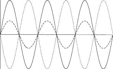
In the special case when k2 equals ÿk1 and ù2 equals ù1 in equation (1.7),

the superposition of the two plane waves becomes
Ø(x, t) ei(kxÿùt) eÿi(kx ùt)	(1:10)
where

k k1 ÿk2

ù ù1 ù2

The two component plane waves in equation (1.10) travel with equal phase velocities ù=k, but in opposite directions. Using equations (A.31) and (A.32), we can express equation (1.10) in the form

Ø(x, t) (eikx eÿikx)eÿiùt

2 cos kx eÿiùt

2 cos kx (cos ùt ÿ i sin ùt)

We see that for this special case the composite wave is the product of two functions: one only of the distance x and the other only of the time t. The composite wave Ø(x, t) vanishes whenever cos kx is zero, i.e., when kx ð=2, 3ð=2, 5ð=2, . . . , regardless of the value of t. Therefore, the nodes of Ø(x, t) are independent of time. However, the amplitude or pro®le of the composite wave changes with time. The real part of Ø(x, t) is shown in Figure 1.3. The solid curve represents the wave when cos ùt is a maximum, the dotted curve when cos ùt is a minimum, and the dashed curve when cos ùt has an intermediate value. Thus, the wave does not travel, but pulsates, increasing and decreasing in amplitude with frequency ù. The imaginary part of Ø(x, t) behaves in the same way. A composite wave with this behavior is known as a standing wave.

8	The wave function

Re Ø(x, t)

x

Figure 1.3 A standing harmonic wave at various times.

1.2 Wave packet

We now consider the formation of a composite wave as the superposition of a continuous spectrum of plane waves with wave numbers k con®ned to a narrow band of values. Such a composite wave Ø(x, t) is known as a wave packet and

may be expressed as
1	1
Ø(x, t) p2ð	…ÿ1 A(k)ei(kxÿùt)dk	(1:11)

••••••

The weighting factor A(k) for each plane wave of wave number k is negligible except when k lies within a small interval Äk. For mathematical convenience we have included a factor (2ð)ÿ1=2 on the right-hand side of equation (1.11). This factor merely changes the value of A(k) and has no other effect.

We note that the wave packet Ø(x, t) is the inverse Fourier transform of A(k). The mathematical development and properties of Fourier transforms are presented in Appendix B. Equation (1.11) has the form of equation (B.19). According to equation (B.20), the Fourier transform A(k) is related to Ø(x, t)

by
1	1	(1:12)
A(k) p2ð	…ÿ1Ø(x, t)eÿi(kxÿùt) dx
••••••

It is because of the Fourier relationships between Ø(x, t) and A(k) that the factor (2ð)ÿ1=2 is included in equation (1.11). Although the time t appears in the integral on the right-hand side of (1.12), the function A(k) does not depend on t; the time dependence of Ø(x, t) cancels the factor eiùt. We consider below

1.2 Wave packet

9

two speci®c examples for the functional form of A(k). However, in order to evaluate the integral over k in equation (1.11), we also need to know the dependence of the angular frequency ù on the wave number k.

In general, the angular frequency ù(k) is a function of k, so that the angular frequencies in the composite wave Ø(x, t), as well as the wave numbers, vary from one plane wave to another. If ù(k) is a slowly varying function of k and the values of k are con®ned to a small range Äk, then ù(k) may be expanded

in a Taylor series in k about some point k0 within the interval Äk
	dù			1	d2ù
ù(k) ù0		0	(k ÿ k0)				0	(k ÿ k0)2	(1:13)
	dk			2		dk2

where ù0 is the value of ù(k) at k0 and the derivatives are also evaluated at k0. We may neglect the quadratic and higher-order terms in the Taylor expansion (1.13) because the interval Äk and, consequently, k ÿ k0 are small. Substitution of equation (1.13) into the phase for each plane wave in (1.11) then gives

				dù
kx ÿ ùt (k ÿ k0 k0)x ÿ ù0 t ÿ						0	(k ÿ k0)t
					dk
k0 x ÿ ù0 t "x ÿ			dk 0 t#(k ÿ k0)
			dù
so that equation (1.11) becomes		B(x, t)ei(k0 xÿù0 t)
Ø(x, t)								(1:14)
where
1	1
B(x, t) p2ð …ÿ1 A(k)ei[xÿ(dù=dk)0 t]( kÿk0) dk								(1:15)

••••••

Thus, the wave packet Ø(x, t) represents a plane wave of wave number k0 and angular frequency ù0 with its amplitude modulated by the factor B(x, t). This modulating function B(x, t) depends on x and t through the relationship [x ÿ (dù=dk)0 t]. This situation is analogous to the case of two plane waves as expressed in equations (1.7) and (1.8). The modulating function B(x, t) moves in the positive x-direction with group velocity vg given by

dù	0
vg dk		(1:16)

In contrast to the group velocity for the two-wave case, as expressed in equation (1.9), the group velocity in (1.16) for the wave packet is not uniquely de®ned. The point k0 is chosen arbitrarily and, therefore, the value at k0 of the derivative dù=dk varies according to that choice. However, the range of k is

10	The wave function

narrow and ù(k) changes slowly with k, so that the variation in vg Combining equations (1.15) and (1.16), we have

1	1
B(x, t) p2ð	…ÿ1 A(k)ei(xÿvg t)(kÿk0) dk
••••••

is small.

(1:17)

Since the function A(k) is the Fourier transform of Ø(x, t), the two functions obey Parseval's theorem as given by equation (B.28) in Appendix B

1	1	1
…ÿ1jØ(x, t)j2dx	…ÿ1jB(x, t)j2 dx	…ÿ1jA(k)j2 dk	(1:18)

Gaussian wave number distribution

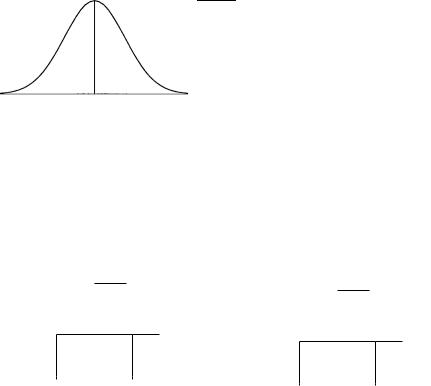
In order to obtain a speci®c mathematical expression for the wave packet, we need to select some form for the function A(k). In our ®rst example we choose A(k) to be the gaussian function

		1	2	=2á	2
A(k)	p2ðá		eÿ(kÿk0)			(1:19)
This function A(k) is a maximum at		••••••		0		, which is also the average
		wave number k

value for k for this distribution of wave numbers. Substitution of equation

(1.19) into (1.17) gives
Ø(x, t)	j	B(x, t)		1	eÿá2(xÿvg t)2=2	(1:20)
j			p
where equation (A.8) has been used. The				••••••
				2ð

resulting modulating factor B(x, t) is also a gaussian function±following the general result that the Fourier transform of a gaussian function is itself gaussian. We have also noted in equation (1.20) that B(x, t) is always positive and is therefore equal to the absolute value jØ(x, t)j of the wave packet. The functions A(k) and jØ(x, t)j are shown in Figure 1.4.

A(k)

1/√

á

|Ø(x, t)|

2ð

1/√2ð

1/√

áe

2ð

1/√2ð e

k

x

(a)

k0 2 √2 á k0 k0 1 √2 á

vg t 2

√2

vg t vg t 1

√2

(b)

á

á

Figure 1.4 (a) A gaussian wave number distribution. (b) The modulating function corresponding to the wave number distribution in Figure 1.4(a).

1.2 Wave packet

11

Figure 1.5 shows the real part of the plane wave exp[i(k0 x ÿ ù0 t)] with its amplitude modulated by B(x, t) of equation (1.20). The plane wave moves in the positive x-direction with phase velocity vph equal to ù0=k0. The maximum amplitude occurs at x vg t and propagates in the positive x-direction with

group velocity vg equal to (dù=dk)0.	p
k0 to 1=e of its maximum value when k ÿ k0j equals			1
	2á. Most		••••••
The value of the function A(k) falls from its maximum value of (			2ðá)ÿ at
p	•••
under the curve (actually 84.3%) comesjfrom the range		of the area
ÿp2á , (k ÿ k0) , p2á
Thus, the distance p2á may •••be regarded as a measure•••	of the width of the

•••

distribution A(k) and is called the half width. The half width may be de®ned using 1=2 or some other fraction instead of 1=e. The reason for using 1=e is that the value of k at that point is easily obtained without consulting a table of numerical values. These various possible de®nitions give different numerical values for the half width, but all these values are of the same order of

magnitude. Since the value of jØ(x, t)j falls from			its maximum value of
(2ð)ÿ	1=2	p	2=á, the distance	p
		to 1=e of that value when x ÿ vg tj equals		2=á
may be considered the half width of jthe wave packet.			•••	•••

When the parameter á is small, the maximum of the function A(k) is high and the function drops off in value rapidly on each side of k0, giving a small value for the half width. The half width of the wave packet, however, is large because it is proportional to 1=á. On the other hand, when the parameter á is large, the maximum of A(k) is low and the function drops off slowly, giving a large half width. In this case, the half width of the wave packet becomes small.

If we regard the uncertainty Äk in the value of k as the half width of the distribution A(k) and the uncertainty Äx in the position of the wave packet as its half width, then the product of these two uncertainties is

ÄxÄk 2

x

Figure 1.5 The real part of a wave packet for a gaussian wave number distribution.